Algorithm Theory: Neural ODE for Cellular Dynamics

Zaoqu Liu

2026-01-26

Introduction

CellODE implements a deep generative model that combines Variational Autoencoders (VAE) with Neural Ordinary Differential Equations (Neural ODE) to infer continuous cellular dynamics from single-cell RNA sequencing data.

This vignette provides a detailed explanation of the mathematical foundations and algorithmic principles underlying CellODE.

Mathematical Framework

Problem Formulation

Given a single-cell gene expression matrix $\mathbf{X} \in \mathbb{R}^{N \times G}$ where $N$ is the number of cells and $G$ is the number of genes, we aim to:

1. Infer a pseudotime $t_i \in [0, 1]$ for each cell $i$
2. Learn a latent representation $\mathbf{z}_i \in \mathbb{R}^d$ capturing cellular state
3. Model the continuous dynamics $\frac{d\mathbf{z}}{dt}$ in latent space

Model Architecture

The TNODE (Time Neural ODE) model consists of three main components:

┌─────────────────────────────────────────────────────────────┐
│                        CellODE Model                         │
├─────────────────────────────────────────────────────────────┤
│                                                             │
│   ┌─────────────┐                                          │
│   │   Input     │  X ∈ ℝ^(N×G)                             │
│   │ Expression  │                                          │
│   └──────┬──────┘                                          │
│          │                                                  │
│          ▼                                                  │
│   ┌─────────────────────────────────────────┐              │
│   │              Encoder Network             │              │
│   │  q(t, z | x) = q(t|x) · q(z|x)         │              │
│   └─────────────────┬───────────────────────┘              │
│                     │                                       │
│          ┌─────────┴─────────┐                             │
│          ▼                   ▼                              │
│   ┌────────────┐      ┌────────────┐                       │
│   │ Time t     │      │ Latent z   │                       │
│   │ (sigmoid)  │      │ (μ, σ²)    │                       │
│   └─────┬──────┘      └──────┬─────┘                       │
│         │                    │                              │
│         └────────────┬───────┘                             │
│                      ▼                                      │
│   ┌─────────────────────────────────────────┐              │
│   │            Neural ODE Solver             │              │
│   │       dz/dt = f_θ(z, t)                 │              │
│   │                                          │              │
│   │  z(t₂) = z(t₁) + ∫_{t₁}^{t₂} f_θ(z,t)dt │              │
│   └─────────────────┬───────────────────────┘              │
│                     │                                       │
│                     ▼                                       │
│   ┌─────────────────────────────────────────┐              │
│   │            Decoder Network               │              │
│   │  p(x | z) ~ NB(μ(z), θ)                 │              │
│   └─────────────────────────────────────────┘              │
│                                                             │
└─────────────────────────────────────────────────────────────┘

Encoder Network

The encoder maps gene expression to time and latent space:

$$q_\phi(t, \mathbf{z} | \mathbf{x}) = q_\phi(t | \mathbf{x}) \cdot q_\phi(\mathbf{z} | \mathbf{x})$$

Time Inference

The time is modeled as a deterministic function with sigmoid activation to constrain values to $[0, 1]$:

$$t = \sigma(f_t(\mathbf{x}))$$

where $\sigma(\cdot)$ is the sigmoid function.

Latent Space Inference

The latent space follows a Gaussian distribution:

$$q_\phi(\mathbf{z} | \mathbf{x}) = \mathcal{N}(\mathbf{z}; \boldsymbol{\mu}_\phi(\mathbf{x}), \text{diag}(\boldsymbol{\sigma}^2_\phi(\mathbf{x})))$$

We use the reparameterization trick for gradient computation:

$$\mathbf{z} = \boldsymbol{\mu} + \boldsymbol{\sigma} \odot \boldsymbol{\epsilon}, \quad \boldsymbol{\epsilon} \sim \mathcal{N}(0, \mathbf{I})$$

Neural ODE

Continuous Dynamics

The core innovation is modeling latent dynamics as a continuous-time process:

$$\frac{d\mathbf{z}(t)}{dt} = f_\theta(\mathbf{z}(t), t)$$

where $f_\theta$ is a neural network parameterized by $\theta$.

Integration

Given initial state $\mathbf{z}_0$ at time $t_0$, the state at any time $t$ is:

$$\mathbf{z}(t) = \mathbf{z}_0 + \int_{t_0}^{t} f_\theta(\mathbf{z}(\tau), \tau) d\tau$$

CellODE uses the Euler method for numerical integration:

$$\mathbf{z}_{n+1} = \mathbf{z}_n + \Delta t \cdot f_\theta(\mathbf{z}_n, t_n)$$

ODE Function Architecture

The latent ODE function $f_\theta$ is implemented as a simple MLP:

Input: z ∈ ℝ^d
    │
    ▼
┌─────────────┐
│ Linear(d→h) │
└─────┬───────┘
      │
      ▼
┌─────────────┐
│    ELU      │
└─────┬───────┘
      │
      ▼
┌─────────────┐
│ Linear(h→d) │
└─────────────┘
      │
      ▼
Output: dz/dt ∈ ℝ^d

Decoder Network

Reconstruction Likelihood

CellODE supports three likelihood models:

1. Negative Binomial (NB)

For UMI count data, the negative binomial distribution is most appropriate:

$$p(x_{ig} | \mathbf{z}_i) = \text{NB}(x_{ig}; \mu_{ig}, \theta_g)$$

where: - $\mu_{ig} = s_i \cdot \text{softmax}(f_\text{dec}(\mathbf{z}_i))_g$ is the expected count - $s_i$ is the library size (total UMI count) - $\theta_g$ is the dispersion parameter

The log-likelihood is:

$$\log p(x | \mu, \theta) = \log\Gamma(x + \theta) - \log\Gamma(\theta) - \log\Gamma(x+1) + \theta\log\frac{\theta}{\theta+\mu} + x\log\frac{\mu}{\theta+\mu}$$

2. Zero-Inflated Negative Binomial (ZINB)

For data with excess zeros:

$$p(x | \mu, \theta, \pi) = \pi \cdot \mathbf{1}_{x=0} + (1-\pi) \cdot \text{NB}(x; \mu, \theta)$$

3. Mean Squared Error (MSE)

For log-normalized data:

$$\mathcal{L}_\text{MSE} = \frac{1}{N}\sum_{i=1}^N ||\mathbf{x}_i - \hat{\mathbf{x}}_i||^2$$

Loss Function

The total loss combines multiple components:

$$\mathcal{L} = \alpha_1 \mathcal{L}_\text{recon}^\text{enc} + \alpha_2 \mathcal{L}_\text{recon}^\text{ode} + \mathcal{L}_\text{z-div} + \alpha_\text{kl} \mathcal{L}_\text{KL}$$

Components

1. Encoder Reconstruction Loss ($\mathcal{L}_\text{recon}^\text{enc}$): Reconstruction from encoder-derived latent space

2. ODE Reconstruction Loss ($\mathcal{L}_\text{recon}^\text{ode}$): Reconstruction from ODE-integrated latent space

3. Latent Divergence ($\mathcal{L}_\text{z-div}$): $$\mathcal{L}_\text{z-div} = ||\mathbf{z}_\text{enc} - \mathbf{z}_\text{ode}||^2$$

4. KL Divergence ($\mathcal{L}_\text{KL}$): $$\mathcal{L}_\text{KL} = \text{KL}[q(\mathbf{z}|\mathbf{x}) || p(\mathbf{z})]$$

   For Gaussian distributions: $$\text{KL} = \frac{1}{2}\sum_{j=1}^d \left(\sigma_j^2 + \mu_j^2 - 1 - \log\sigma_j^2\right)$$

Time Direction Determination

The model may learn pseudotime in either direction. CellODE automatically determines the correct direction using the correlation between inferred time and number of detected genes:

$$\beta = \text{cov}(t, \log(n_\text{genes}))$$

If $\beta > 0$, the time is reversed since more mature cells typically have fewer detected genes.

Demonstration

Let’s visualize how the Neural ODE models dynamics:

library(torch)

# Create a simple ODE function
ode_func <- torch::nn_module(
  initialize = function() {
    self$fc1 <- torch::nn_linear(2, 32)
    self$fc2 <- torch::nn_linear(32, 2)
  },
  forward = function(t, z) {
    out <- torch::nnf_elu(self$fc1(z))
    self$fc2(out)
  }
)

# Initialize
func <- ode_func()
torch::torch_manual_seed(42)

# Create initial points on a circle
n_points <- 20
theta <- seq(0, 2*pi, length.out = n_points + 1)[1:n_points]
z0 <- torch::torch_stack(list(
  torch::torch_tensor(0.5 * cos(theta)),
  torch::torch_tensor(0.5 * sin(theta))
), dim = 2)

# Time points
t <- torch::torch_linspace(0, 1, 20)

# Simple Euler integration
func$eval()
trajectories <- list()

torch::with_no_grad({
  for (i in 1:n_points) {
    z <- z0[i, ]
    traj <- matrix(0, nrow = 20, ncol = 2)
    traj[1, ] <- as.numeric(z)
    
    for (j in 2:20) {
      dt <- (t[j] - t[j-1])$item()
      dz <- func(t[j-1], z)
      z <- z + dt * dz
      traj[j, ] <- as.numeric(z)
    }
    trajectories[[i]] <- traj
  }
})

# Plot trajectories
plot(NULL, xlim = c(-1.5, 1.5), ylim = c(-1.5, 1.5),
     xlab = "z1", ylab = "z2", main = "Neural ODE Trajectories")

colors <- rainbow(n_points)
for (i in 1:n_points) {
  lines(trajectories[[i]], col = colors[i], lwd = 1.5)
  points(trajectories[[i]][1, 1], trajectories[[i]][1, 2], 
         pch = 19, col = colors[i], cex = 1)
  points(trajectories[[i]][20, 1], trajectories[[i]][20, 2], 
         pch = 17, col = colors[i], cex = 1)
}
legend("topright", legend = c("Start", "End"), pch = c(19, 17), bty = "n")

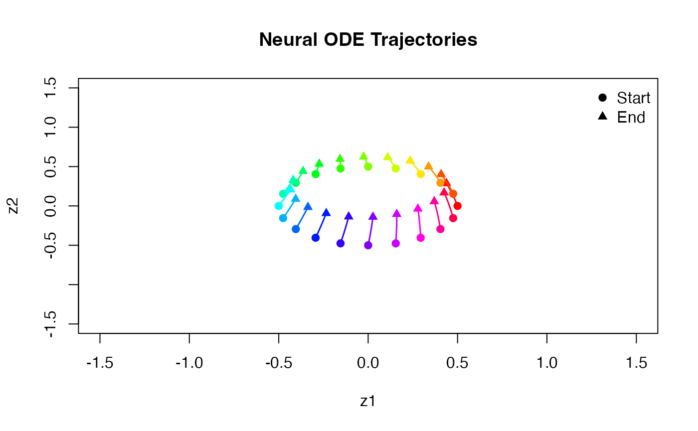
Key Innovations

1. Automatic Time Inference

Unlike methods requiring specification of root cells, CellODE infers pseudotime directly from the data through the encoder network.

2. Continuous Dynamics

The Neural ODE framework provides: - Continuous (not discrete) state transitions - Physically interpretable dynamics (velocity field) - Memory-efficient training via adjoint method

3. Unified Framework

CellODE jointly learns: - Temporal ordering (pseudotime) - Low-dimensional representation (latent space) - Dynamical model (vector field)

References

1. Li, S. et al. (2023). scTour: a deep learning architecture for robust inference and accurate prediction of cellular dynamics. Genome Biology, 24, 149.

2. Chen, R.T.Q. et al. (2018). Neural Ordinary Differential Equations. NeurIPS.

3. Kingma, D.P. & Welling, M. (2014). Auto-Encoding Variational Bayes. ICLR.

4. Lopez, R. et al. (2018). Deep generative modeling for single-cell transcriptomics. Nature Methods, 15, 1053-1058.

Session Info

sessionInfo()