Introduction
NOVA provides a comprehensive suite of visualization functions to explore and present cell-cell communication analysis results. This gallery demonstrates the various plotting capabilities with practical examples.
Setup
Creating Example Data
set.seed(123)

# Simulate expression matrix
n_genes <- 200
n_cells <- 500
gene_names <- paste0("Gene", 1:n_genes)
cell_names <- paste0("Cell", 1:n_cells)

expr <- matrix(0, nrow = n_genes, ncol = n_cells,
               dimnames = list(gene_names, cell_names))
expressed <- sample(length(expr), size = length(expr) * 0.25)
expr[expressed] <- abs(rnorm(length(expressed), mean = 3, sd = 1.5))
expr <- Matrix::Matrix(expr, sparse = TRUE)

# Create clusters
clusters <- sample(c("T_cells", "B_cells", "Macrophages", "Fibroblasts", "Dendritic"),
                   n_cells, replace = TRUE, prob = c(0.25, 0.20, 0.25, 0.15, 0.15))
names(clusters) <- cell_names
annotation <- data.frame(cell = cell_names, cluster = clusters)

# Map genes to LR database
lr_db <- GetLRDatabase("lrc2p")
ligands <- unique(lr_db$ligand)[1:30]
receptors <- unique(lr_db$receptor)[1:30]
rownames(expr)[1:30] <- ligands
rownames(expr)[31:60] <- receptors
Running Analysis
# Run NOVA analysis
result <- ExtractEdges(
  expression = expr,
  annotation = annotation,
  species = "human",
  database = "lrc2p",
  min_pct = 0.05
)

print(result)
1. Communication Heatmap
The heatmap displays the overall communication strength between cell types.
Basic Heatmap
# Count-based heatmap
ht <- PlotHeatmap(result, metric = "count", show_values = TRUE)
Specificity-weighted Heatmap
# Specificity-based heatmap
ht_spec <- PlotHeatmap(result, metric = "specificity", show_values = TRUE)
2. Network Visualization
Network graphs provide an intuitive view of communication patterns.
Circular Layout
PlotNetwork(result,
            layout = "circle",
            metric = "count",
            title = "Cell-Cell Communication Network")
Force-directed Layout
PlotNetwork(result,
            layout = "fr",  # Fruchterman-Reingold
            metric = "specificity",
            title = "Communication Network (FR Layout)")
Kamada-Kawai Layout
PlotNetwork(result,
            layout = "kk",
            metric = "count",
            title = "Communication Network (KK Layout)")
3. Chord Diagram
Chord diagrams elegantly display the flow of communication between cell types.
PlotChord(result,
          metric = "count",
          transparency = 0.4,
          title = "Communication Flow")
Specificity-based Chord
PlotChord(result,
          metric = "specificity",
          transparency = 0.5,
          title = "Specificity-weighted Communication")
4. Ligand-Receptor Pairs Visualization
Examine specific LR pairs between cluster pairs.
# Get specific cluster pair interactions
PlotLRPairs(result,
            sending = "T_cells",
            target = "Macrophages",
            top_n = 15,
            rank_by = "specificity",
            title = "T cells → Macrophages LR Interactions")
PlotLRPairs(result,
            sending = "Macrophages",
            target = "Fibroblasts",
            top_n = 10,
            rank_by = "mean")
5. Color Palette
NOVA provides a custom color palette optimized for cell type visualization.
# Display color palette
colors <- nova_palette(20)
barplot(rep(1, 20), col = colors, border = NA, axes = FALSE,
        main = "NOVA Color Palette")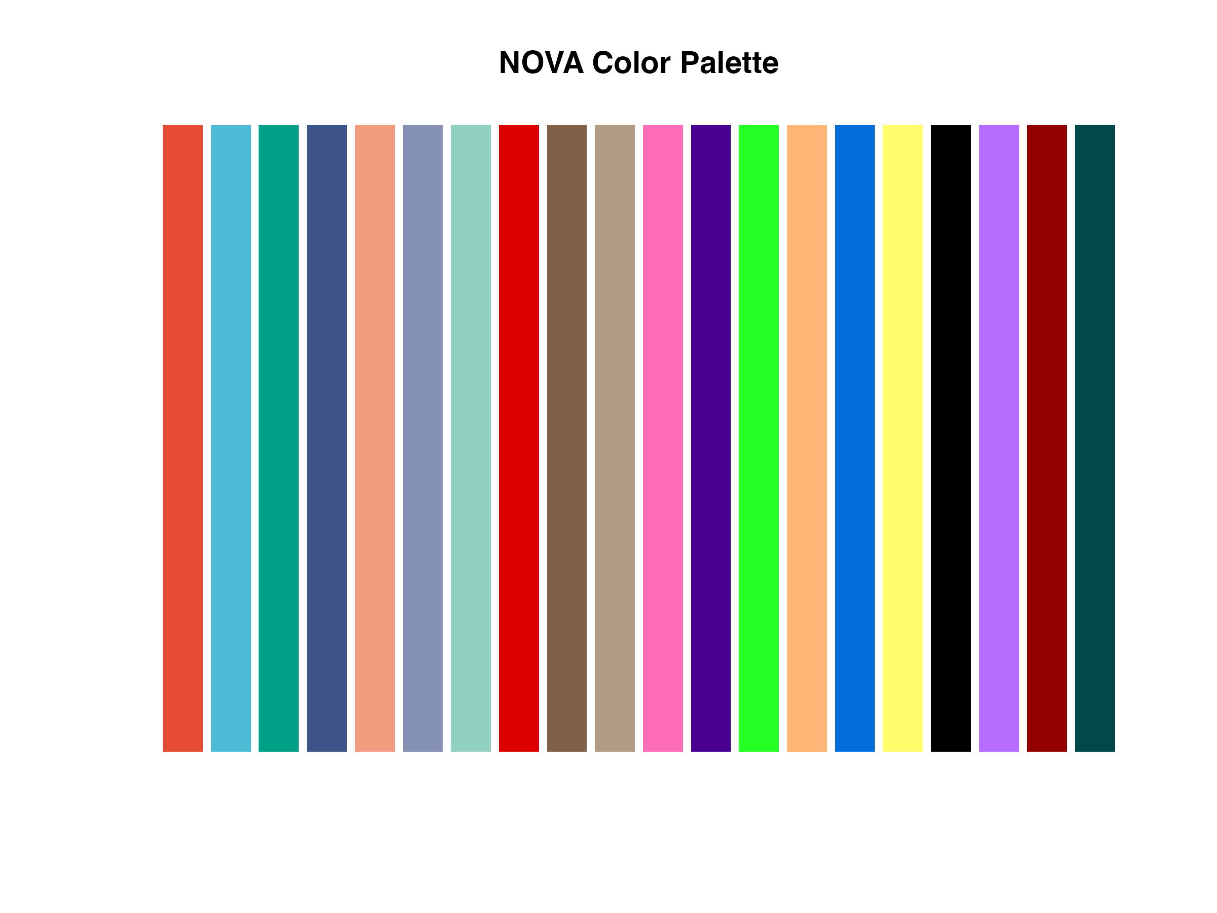
NOVA color palette
6. Custom Styling
Custom Colors
custom_cols <- c("T_cells" = "#E64B35",
                 "B_cells" = "#4DBBD5",
                 "Macrophages" = "#00A087",
                 "Fibroblasts" = "#3C5488",
                 "Dendritic" = "#F39B7F")

PlotNetwork(result,
            layout = "circle",
            colors = custom_cols,
            title = "Network with Custom Colors")
7. Saving Plots
# Save heatmap to PDF
SavePlot(ht, "communication_heatmap.pdf", width = 10, height = 8)

# Save network to PNG
p <- PlotNetwork(result, layout = "circle")
SavePlot(p, "communication_network.png", width = 10, height = 8, dpi = 300)
Summary Table
| Function | Description | Output Type |
|---|---|---|
PlotHeatmap() |
Communication strength heatmap | ComplexHeatmap |
PlotNetwork() |
Network graph | ggplot2 |
PlotChord() |
Chord diagram | Base R |
PlotLRPairs() |
Bipartite LR visualization | ggplot2 |
PlotDiffHeatmap() |
Differential communication heatmap | ComplexHeatmap |
PlotVolcano() |
Volcano plot | ggplot2 |
Session Info
sessionInfo()
#> R version 4.4.0 (2024-04-24)
#> Platform: aarch64-apple-darwin20
#> Running under: macOS 15.6.1
#>
#> Matrix products: default
#> BLAS:   /Library/Frameworks/R.framework/Versions/4.4-arm64/Resources/lib/libRblas.0.dylib
#> LAPACK: /Library/Frameworks/R.framework/Versions/4.4-arm64/Resources/lib/libRlapack.dylib;  LAPACK version 3.12.0
#>
#> locale:
#> [1] C
#>
#> time zone: Asia/Shanghai
#> tzcode source: internal
#>
#> attached base packages:
#> [1] stats     graphics  grDevices utils     datasets  methods   base
#>
#> other attached packages:
#> [1] ggplot2_4.0.1 NOVA_1.0.0
#>
#> loaded via a namespace (and not attached):
#>  [1] Matrix_1.7-4       gtable_0.3.6       jsonlite_2.0.0     dplyr_1.1.4
#>  [5] compiler_4.4.0     Rcpp_1.1.1         tidyselect_1.2.1   parallel_4.4.0
#>  [9] dichromat_2.0-0.1  jquerylib_0.1.4    systemfonts_1.3.1  scales_1.4.0
#> [13] textshaping_1.0.4  yaml_2.3.12        fastmap_1.2.0      lattice_0.22-7
#> [17] R6_2.6.1           generics_0.1.4     knitr_1.51         htmlwidgets_1.6.4
#> [21] tibble_3.3.1       desc_1.4.3         bslib_0.9.0        pillar_1.11.1
#> [25] RColorBrewer_1.1-3 rlang_1.1.7        cachem_1.1.0       xfun_0.56
#> [29] fs_1.6.6           sass_0.4.10        S7_0.2.1           otel_0.2.0
#> [33] cli_3.6.5          withr_3.0.2        pkgdown_2.2.0      magrittr_2.0.4
#> [37] digest_0.6.39      grid_4.4.0         lifecycle_1.0.5    vctrs_0.7.1
#> [41] data.table_1.18.0  evaluate_1.0.5     glue_1.8.0         farver_2.1.2
#> [45] ragg_1.5.0         rmarkdown_2.30     tools_4.4.0        pkgconfig_2.0.3
#> [49] htmltools_0.5.9