LIANA Algorithm Principles and Mathematical Framework

Overview

LIANA (LIgand-receptor ANalysis frAmework) integrates multiple cell-cell communication (CCC) inference methods. This vignette provides a comprehensive mathematical description of each scoring algorithm implemented in LIANA.

Cell-Cell Communication Inference

The fundamental premise of CCC inference from scRNA-seq data is that the expression levels of ligand genes in “sender” cells and receptor genes in “receiver” cells can indicate potential intercellular signaling.

For a ligand $L$ expressed in cell type $A$ and receptor $R$ expressed in cell type $B$ , we seek to quantify:

Expression Magnitude: How strongly are $L$ and $R$ expressed?
Expression Specificity: How specific is this $L$ - $R$ interaction to the $A$ - $B$ cell type pair?

Scoring Methods

1. SingleCellSignalR (LRScore)

Mathematical Formulation

The LRScore from SingleCellSignalR is a dataset-independent score bounded between 0 and 1:

$\text{LRScore} = \frac{\sqrt{\bar{x}_L} \cdot \sqrt{\bar{x}_R}}{\mu_g + \sqrt{\bar{x}_L} \cdot \sqrt{\bar{x}_R}}$

Where: - $\bar{x}_L$ = mean expression of ligand $L$ in source cell type - $\bar{x}_R$ = mean expression of receptor $R$ in target cell type
- $\mu_g$ = global mean expression across all genes and cells

Interpretation

Range: [0, 1]
Higher is better: Higher scores indicate stronger expression
Dataset-independent: Comparable across different datasets

2. NATMI (Edge Specificity)

Mathematical Formulation

NATMI calculates specificity-weighted edge scores:

$\text{Specificity} = \frac{\bar{x}_L}{\sum_c \bar{x}_{L,c}} \times \frac{\bar{x}_R}{\sum_c \bar{x}_{R,c}}$

Where: - $\sum_c \bar{x}_{L,c}$ = sum of ligand expression across all cell types - $\sum_c \bar{x}_{R,c}$ = sum of receptor expression across all cell types

Interpretation

Range: [0, 1]
Higher is better: Score of 1 indicates both ligand and receptor are exclusively expressed in the given cell type pair
Specificity-focused: Prioritizes cell-type specific interactions

Mathematical Insight

The specificity score can be decomposed as:

$\text{Specificity} = P(L|A) \times P(R|B)$

Where $P(L|A)$ is the proportion of ligand expression attributed to cell type $A$ .

3. Connectome (Scaled Weights)

Mathematical Formulation

Connectome uses z-score scaled expression:

$\text{weight\_sc} = \frac{z_L + z_R}{2}$

Where the z-score is calculated as:

$z_g = \frac{\bar{x}_g - \mu_g}{\sigma_g}$

$\mu_g$ = mean expression of gene $g$ across cell types
$\sigma_g$ = standard deviation of gene $g$ across cell types

Interpretation

Range: Unbounded (can be negative)
Higher is better: Higher z-scores indicate above-average expression
Relative measure: Compares expression to the overall distribution

4. CellPhoneDB (Permutation-based P-values)

Mathematical Formulation

CellPhoneDB uses a permutation-based approach:

Calculate the observed mean: $\bar{x}_{LR} = \frac{\bar{x}_L + \bar{x}_R}{2}$
Generate null distribution by permuting cell type labels $n$ times
Calculate p-value: $p = \frac{\#\{\bar{x}_{LR}^{perm} \geq \bar{x}_{LR}^{obs}\}}{n_{perms}}$

Interpretation

Range: [0, 1]
Lower is better: Low p-values indicate interactions unlikely to occur by chance
Statistical rigor: Controls for dataset-specific expression patterns

5. LogFC Method

Mathematical Formulation

The logFC method uses fold-change between cell types:

$\text{logFC}_L = \log_2\left(\frac{\bar{x}_{L,A} + 1}{\bar{x}_{L,\text{other}} + 1}\right)$

Combined score:

$\text{logfc\_comb} = \frac{\text{logFC}_L + \text{logFC}_R}{2}$

Interpretation

Range: Unbounded
Higher is better: Positive values indicate enrichment in the cell type pair
Differential expression: Captures cell-type enriched interactions

6. CytoTalk (Crosstalk Score)

Mathematical Formulation

CytoTalk combines expression scores (ES) with non-self-talk scores (NST):

Preferential Expression Measure (PEM): $\text{PEM}_{g,c} = \log_{10}\left(\frac{\bar{x}_{g,c}}{E[\bar{x}_{g,c}]}\right)$
Non-Self-Talk Score (based on mutual information): $\text{NST} = -\log_{10}\left(\frac{MI(L, R)}{\min(H_L, H_R)}\right)$
Final Crosstalk Score: $\text{Crosstalk} = \begin{cases} \text{Nes} \times \text{Nnst} & \text{if paracrine} \\ \text{Nes} \times (1 - \text{Nnst}) & \text{if autocrine} \end{cases}$

Where $\text{Nes}$ and $\text{Nnst}$ are min-max normalized scores.

Consensus Ranking

Robust Rank Aggregation (RRA)

LIANA uses RRA to combine rankings from multiple methods:

$\rho(r) = \min_{1 \leq k \leq K} \beta_{k,n}(r_k)$

Where $\beta_{k,n}$ is the probability of observing a rank $r_k$ or better in a random ordering.

Properties

Robust to outliers: Uses order statistics
Statistically principled: Based on order statistics of uniform distribution
P-value interpretation: Low aggregate rank indicates consistent high ranking

Complex Handling

For heteromeric complexes (e.g., $L_1\_L_2$ interacting with $R_1\_R_2$ ), LIANA applies a policy function:

$\text{Complex Score} = f(\{s_1, s_2, ..., s_n\})$

Available policies: - mean0: Mean, but returns 0 if any subunit is absent - min: Minimum subunit score (limiting factor) - geometric_mean: Geometric mean of subunits

Visualization of Score Distributions

library(liana)
library(ggplot2)
library(dplyr)
library(tidyr)

# Load example data
liana_path <- system.file(package = "liana")
testdata <- readRDS(file.path(liana_path, "testdata", "input", "testdata.rds"))

# Run LIANA
liana_res <- liana_wrap(testdata, 
                        method = c("natmi", "sca", "connectome", "logfc"),
                        resource = "Consensus")

# Aggregate results
liana_aggr <- liana_aggregate(liana_res)

# Visualize score distributions
liana_aggr %>%
  select(ends_with("rank")) %>%
  pivot_longer(everything(), names_to = "Method", values_to = "Rank") %>%
  mutate(Method = gsub("\\.rank", "", Method)) %>%
  ggplot(aes(x = Rank, fill = Method)) +
  geom_density(alpha = 0.5) +
  theme_minimal(base_size = 12) +
  labs(title = "Distribution of Ranks Across Methods",
       x = "Rank", y = "Density") +
  theme(legend.position = "bottom")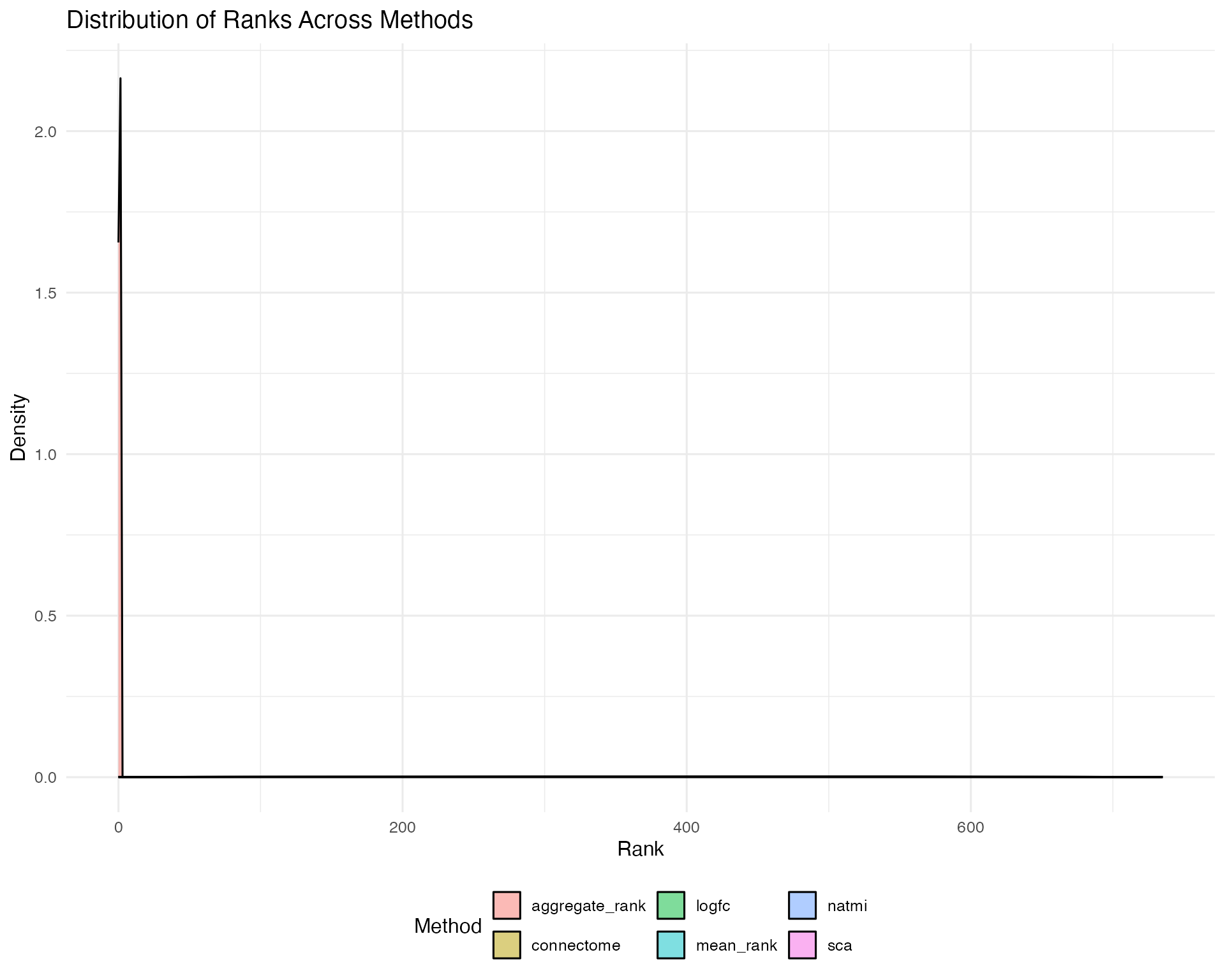

Score Correlation Heatmap

# Calculate correlations between method scores
score_cols <- liana_aggr %>%
  select(ends_with("rank")) %>%
  cor(use = "complete.obs")

# Plot correlation heatmap
score_cols %>%
  as.data.frame() %>%
  tibble::rownames_to_column("Method1") %>%
  pivot_longer(-Method1, names_to = "Method2", values_to = "Correlation") %>%
  mutate(Method1 = gsub("\\.rank", "", Method1),
         Method2 = gsub("\\.rank", "", Method2)) %>%
  ggplot(aes(x = Method1, y = Method2, fill = Correlation)) +
  geom_tile() +
  geom_text(aes(label = round(Correlation, 2)), color = "white", size = 5) +
  scale_fill_gradient2(low = "blue", mid = "white", high = "red", midpoint = 0.5) +
  theme_minimal(base_size = 12) +
  labs(title = "Rank Correlation Between Methods",
       x = "", y = "") +
  theme(axis.text.x = element_text(angle = 45, hjust = 1))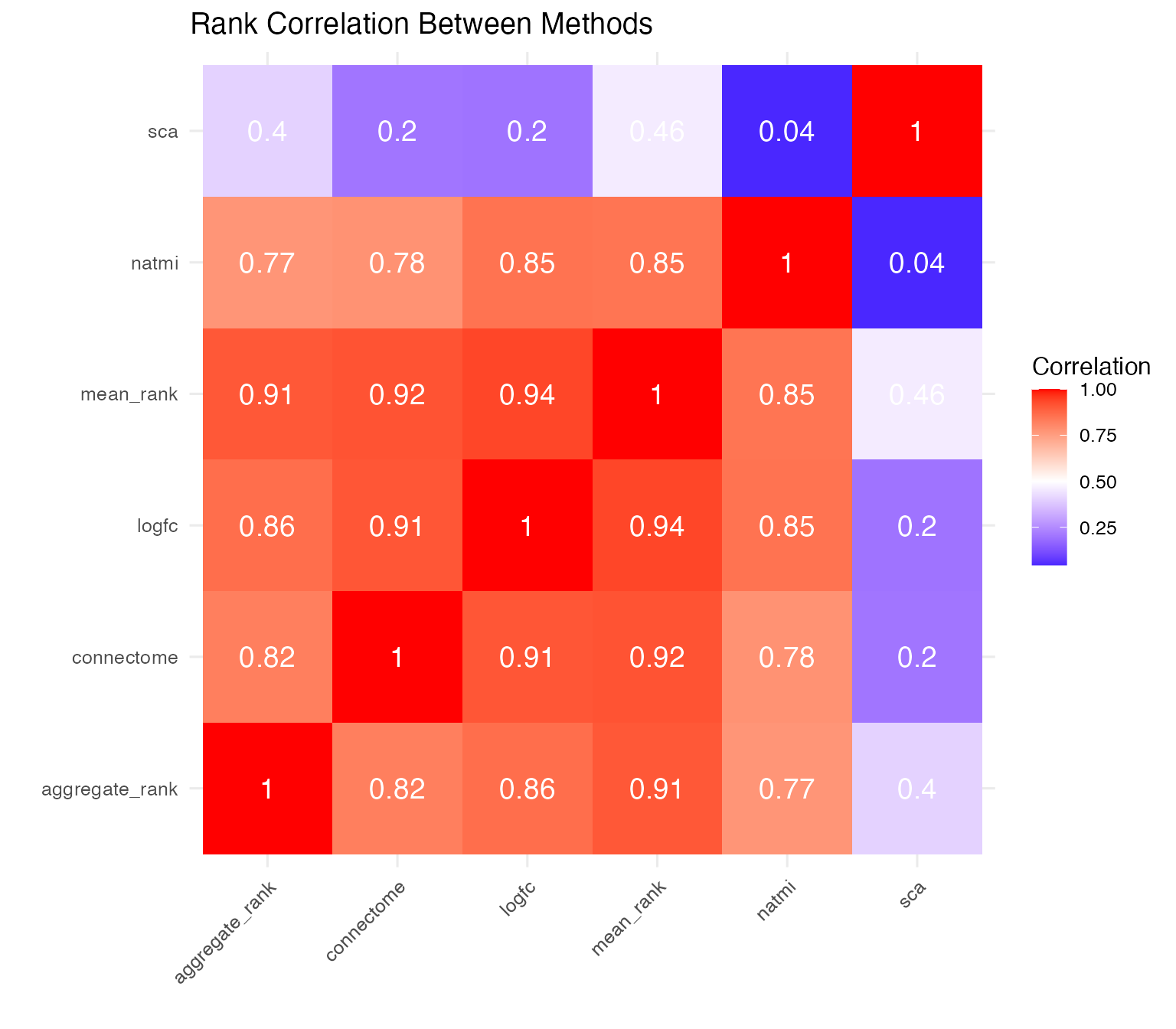

Summary Table

Method	Score Type	Range	Interpretation	Best For
SingleCellSignalR	Magnitude	[0,1]	Higher = stronger	Cross-dataset comparison
NATMI	Specificity	[0,1]	Higher = more specific	Cell-type specific interactions
Connectome	Z-score	Unbounded	Higher = enriched	Relative expression
CellPhoneDB	P-value	[0,1]	Lower = significant	Statistical validation
LogFC	Fold-change	Unbounded	Higher = enriched	Differential interactions
CytoTalk	Crosstalk	[0,1]	Higher = stronger	Autocrine/paracrine distinction

References

Dimitrov D, et al. (2022). Comparison of methods and resources for cell-cell communication inference from single-cell RNA-Seq data. Nature Communications.
Cabello-Aguilar S, et al. (2020). SingleCellSignalR: inference of intercellular networks from single-cell transcriptomics. Nucleic Acids Research.
Hou R, et al. (2020). Predicting cell-to-cell communication networks using NATMI. Nature Communications.
Raredon MSB, et al. (2019). Single-cell connectomic analysis of adult mammalian lungs. Science Advances.
Efremova M, et al. (2020). CellPhoneDB: inferring cell–cell communication from combined expression of multi-subunit ligand–receptor complexes. Nature Protocols.

Session Information

#> R version 4.4.0 (2024-04-24)
#> Platform: aarch64-apple-darwin20
#> Running under: macOS 15.6.1
#> 
#> Matrix products: default
#> BLAS:   /Library/Frameworks/R.framework/Versions/4.4-arm64/Resources/lib/libRblas.0.dylib 
#> LAPACK: /Library/Frameworks/R.framework/Versions/4.4-arm64/Resources/lib/libRlapack.dylib;  LAPACK version 3.12.0
#> 
#> locale:
#> [1] C
#> 
#> time zone: Asia/Shanghai
#> tzcode source: internal
#> 
#> attached base packages:
#> [1] stats     graphics  grDevices utils     datasets  methods   base     
#> 
#> other attached packages:
#> [1] tidyr_1.3.2       dplyr_1.1.4       ggplot2_4.0.1     liana_0.1.14.9000
#> [5] BiocStyle_2.34.0 
#> 
#> loaded via a namespace (and not attached):
#>   [1] spatstat.sparse_3.1-0       fs_1.6.6                   
#>   [3] matrixStats_1.5.0           lubridate_1.9.4            
#>   [5] httr_1.4.7                  RColorBrewer_1.1-3         
#>   [7] doParallel_1.0.17           tools_4.4.0                
#>   [9] sctransform_0.4.3           backports_1.5.0            
#>  [11] R6_2.6.1                    uwot_0.2.4                 
#>  [13] lazyeval_0.2.2              GetoptLong_1.1.0           
#>  [15] withr_3.0.2                 sp_2.2-0                   
#>  [17] gridExtra_2.3               prettyunits_1.2.0          
#>  [19] progressr_0.18.0            cli_3.6.5                  
#>  [21] Biobase_2.66.0              textshaping_1.0.4          
#>  [23] spatstat.explore_3.6-0      labeling_0.4.3             
#>  [25] sass_0.4.10                 Seurat_4.4.0               
#>  [27] spatstat.data_3.1-9         S7_0.2.1                   
#>  [29] readr_2.1.6                 ggridges_0.5.7             
#>  [31] pbapply_1.7-4               pkgdown_2.1.3              
#>  [33] systemfonts_1.3.1           R.utils_2.13.0             
#>  [35] scater_1.34.1               dichromat_2.0-0.1          
#>  [37] parallelly_1.46.1           sessioninfo_1.2.3          
#>  [39] limma_3.62.2                readxl_1.4.5               
#>  [41] RSQLite_2.4.5               generics_0.1.4             
#>  [43] shape_1.4.6.1               spatstat.random_3.4-3      
#>  [45] ica_1.0-3                   zip_2.3.3                  
#>  [47] Matrix_1.7-4                ggbeeswarm_0.7.3           
#>  [49] S4Vectors_0.44.0            logger_0.4.1               
#>  [51] abind_1.4-8                 R.methodsS3_1.8.2          
#>  [53] lifecycle_1.0.5             yaml_2.3.12                
#>  [55] edgeR_4.4.2                 SummarizedExperiment_1.36.0
#>  [57] SparseArray_1.6.2           Rtsne_0.17                 
#>  [59] grid_4.4.0                  blob_1.2.4                 
#>  [61] promises_1.5.0              dqrng_0.4.1                
#>  [63] crayon_1.5.3                dir.expiry_1.14.0          
#>  [65] miniUI_0.1.2                lattice_0.22-7             
#>  [67] beachmat_2.22.0             cowplot_1.2.0              
#>  [69] chromote_0.5.1              pillar_1.11.1              
#>  [71] knitr_1.51                  ComplexHeatmap_2.22.0      
#>  [73] metapod_1.14.0              GenomicRanges_1.58.0       
#>  [75] tcltk_4.4.0                 rjson_0.2.23               
#>  [77] future.apply_1.20.1         codetools_0.2-20           
#>  [79] leiden_0.4.3.1              glue_1.8.0                 
#>  [81] spatstat.univar_3.1-6       data.table_1.18.0          
#>  [83] vctrs_0.7.0                 png_0.1-8                  
#>  [85] cellranger_1.1.0            gtable_0.3.6               
#>  [87] cachem_1.1.0                OmnipathR_3.19.1           
#>  [89] xfun_0.56                   S4Arrays_1.6.0             
#>  [91] mime_0.13                   survival_3.8-3             
#>  [93] SingleCellExperiment_1.28.1 iterators_1.0.14           
#>  [95] statmod_1.5.1               bluster_1.16.0             
#>  [97] fitdistrplus_1.2-4          ROCR_1.0-11                
#>  [99] nlme_3.1-168                bit64_4.6.0-1              
#> [101] progress_1.2.3              filelock_1.0.3             
#> [103] RcppAnnoy_0.0.23            GenomeInfoDb_1.42.3        
#> [105] bslib_0.9.0                 irlba_2.3.5.1              
#> [107] vipor_0.4.7                 KernSmooth_2.23-26         
#> [109] otel_0.2.0                  colorspace_2.1-2           
#> [111] BiocGenerics_0.52.0         DBI_1.2.3                  
#> [113] tidyselect_1.2.1            processx_3.8.6             
#> [115] bit_4.6.0                   compiler_4.4.0             
#> [117] curl_7.0.0                  rvest_1.0.5                
#> [119] httr2_1.2.2                 BiocNeighbors_2.0.1        
#> [121] xml2_1.5.2                  desc_1.4.3                 
#> [123] DelayedArray_0.32.0         plotly_4.11.0              
#> [125] bookdown_0.44               checkmate_2.3.3            
#> [127] scales_1.4.0                lmtest_0.9-40              
#> [129] rappdirs_0.3.4              goftest_1.2-3              
#> [131] stringr_1.6.0               digest_0.6.39              
#> [133] spatstat.utils_3.2-1        rmarkdown_2.30             
#> [135] basilisk_1.23.0             XVector_0.46.0             
#> [137] htmltools_0.5.9             pkgconfig_2.0.3            
#> [139] sparseMatrixStats_1.18.0    MatrixGenerics_1.18.1      
#> [141] fastmap_1.2.0               rlang_1.1.7                
#> [143] GlobalOptions_0.1.3         htmlwidgets_1.6.4          
#> [145] UCSC.utils_1.2.0            shiny_1.12.1               
#> [147] farver_2.1.2                jquerylib_0.1.4            
#> [149] zoo_1.8-15                  jsonlite_2.0.0             
#> [151] BiocParallel_1.40.2         R.oo_1.27.1                
#> [153] BiocSingular_1.22.0         magrittr_2.0.4             
#> [155] scuttle_1.16.0              GenomeInfoDbData_1.2.13    
#> [157] patchwork_1.3.2             Rcpp_1.1.1                 
#> [159] viridis_0.6.5               reticulate_1.44.1          
#> [161] stringi_1.8.7               zlibbioc_1.52.0            
#> [163] MASS_7.3-65                 plyr_1.8.9                 
#> [165] parallel_4.4.0              listenv_0.10.0             
#> [167] ggrepel_0.9.6               deldir_2.0-4               
#> [169] splines_4.4.0               tensor_1.5.1               
#> [171] hms_1.1.4                   circlize_0.4.17            
#> [173] locfit_1.5-9.12             ps_1.9.1                   
#> [175] igraph_2.2.1                spatstat.geom_3.6-1        
#> [177] reshape2_1.4.5              stats4_4.4.0               
#> [179] ScaledMatrix_1.14.0         XML_3.99-0.20              
#> [181] evaluate_1.0.5              SeuratObject_4.1.4         
#> [183] scran_1.34.0                BiocManager_1.30.27        
#> [185] tzdb_0.5.0                  foreach_1.5.2              
#> [187] httpuv_1.6.16               polyclip_1.10-7            
#> [189] RANN_2.6.2                  purrr_1.2.1                
#> [191] future_1.69.0               clue_0.3-66                
#> [193] scattermore_1.2             rsvd_1.0.5                 
#> [195] xtable_1.8-4                later_1.4.5                
#> [197] viridisLite_0.4.2           ragg_1.5.0                 
#> [199] tibble_3.3.1                websocket_1.4.4            
#> [201] beeswarm_0.4.0              memoise_2.0.1              
#> [203] IRanges_2.40.1              cluster_2.1.8.1            
#> [205] timechange_0.3.0            globals_0.18.0

Zaoqu Liu

Daniel Dimitrov

2026-01-23

Overview

Cell-Cell Communication Inference

Scoring Methods

1. SingleCellSignalR (LRScore)

Mathematical Formulation

Interpretation

2. NATMI (Edge Specificity)

Mathematical Formulation

Interpretation

Mathematical Insight

3. Connectome (Scaled Weights)

Mathematical Formulation

Interpretation

4. CellPhoneDB (Permutation-based P-values)

Mathematical Formulation

Interpretation

5. LogFC Method

Mathematical Formulation

Interpretation

6. CytoTalk (Crosstalk Score)

Mathematical Formulation

Consensus Ranking

Robust Rank Aggregation (RRA)

Properties

Complex Handling

Visualization of Score Distributions

Score Correlation Heatmap

Summary Table

References

Session Information