LIANA Visualization Guide
Zaoqu Liu
Fork Maintainerliuzaoqu@163.com
2026-01-23
Source:vignettes/visualization.Rmd
visualization.RmdOverview
This vignette demonstrates various visualization options available in LIANA for exploring cell-cell communication results.
Run LIANA Analysis
# Run analysis
liana_res <- liana_wrap(testdata,
  method = c("natmi", "connectome", "logfc", "sca"),
  resource = "Consensus"
)

# Aggregate results
liana_aggr <- liana_aggregate(liana_res)
1. Dotplot Visualizations
Basic Dotplot
The dotplot is the primary visualization for LIANA results, showing: - Color: Expression magnitude (LRscore) - Size: Interaction specificity (edge_specificity)
liana_aggr %>%
  liana_dotplot(ntop = 20)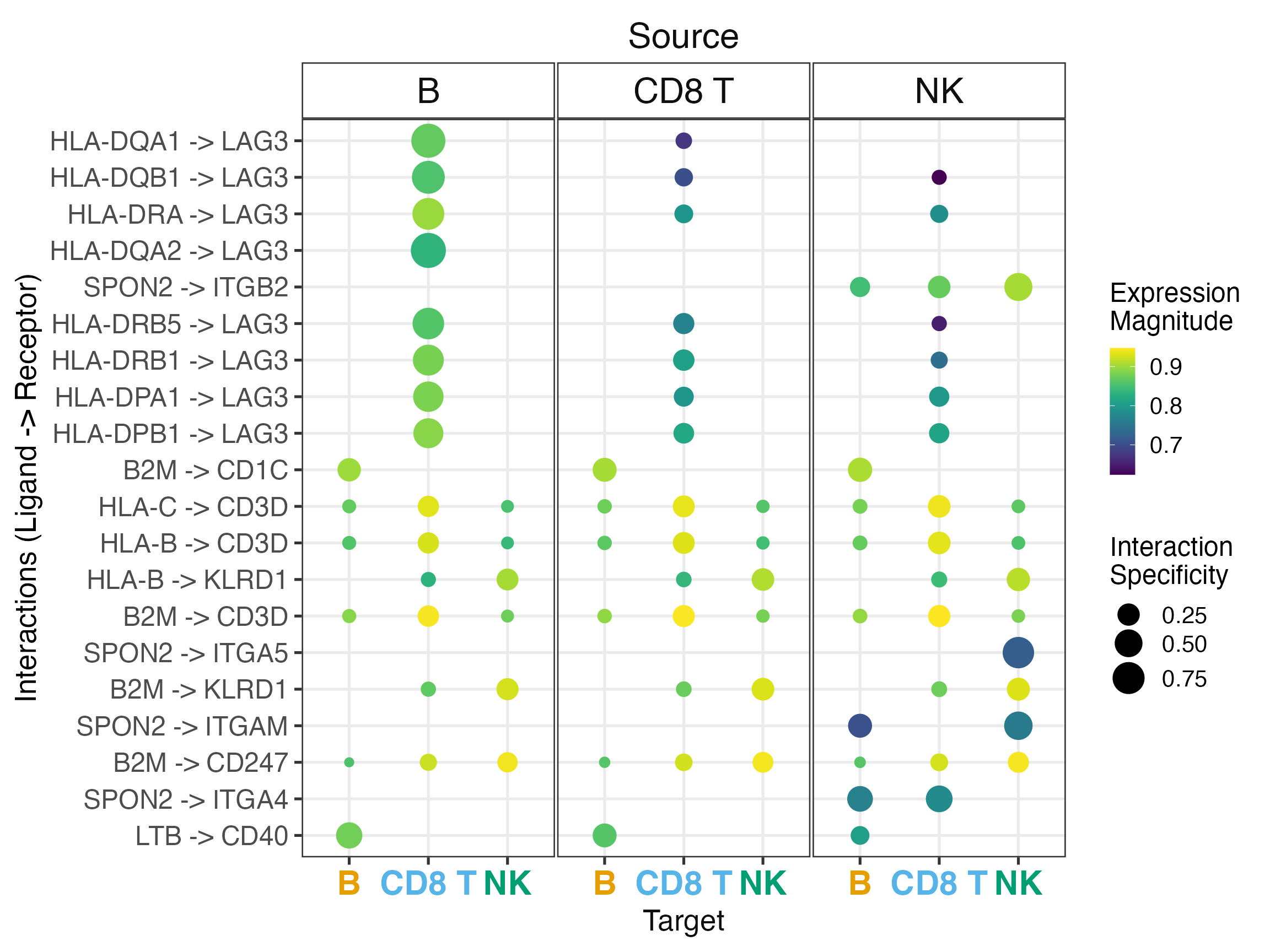
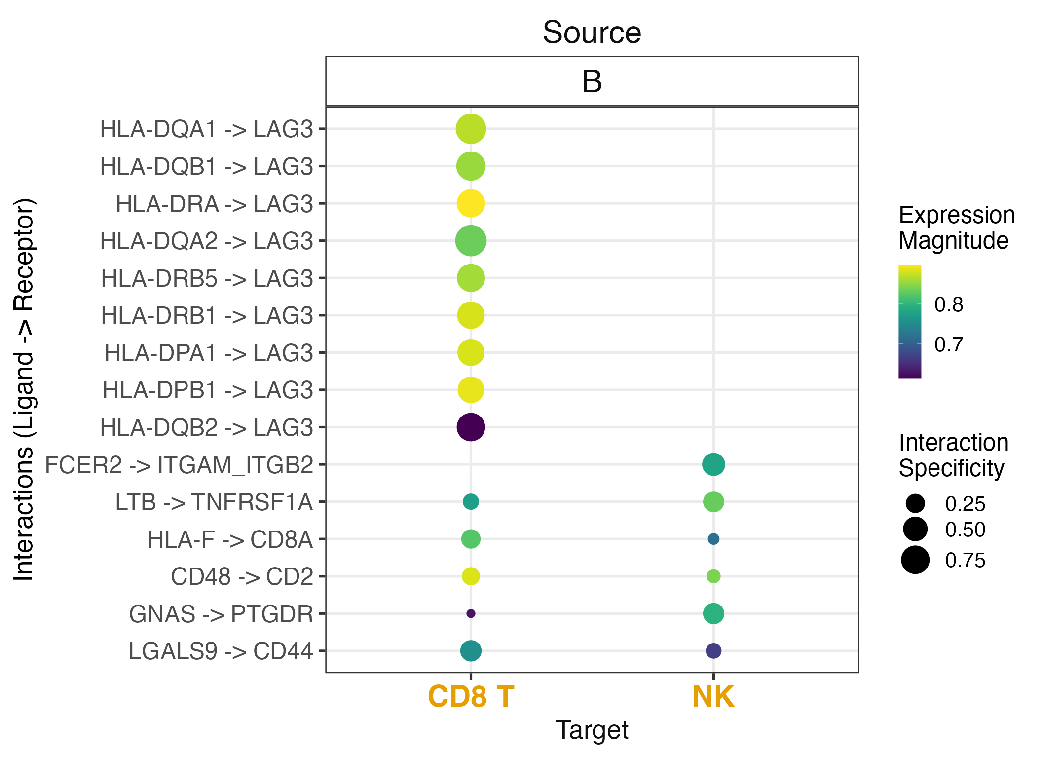
Filtered Dotplot
# Filter by source and target cell types
liana_aggr %>%
  liana_dotplot(
    source_groups = c("B"),
    target_groups = c("NK", "CD8 T"),
    ntop = 15
  )
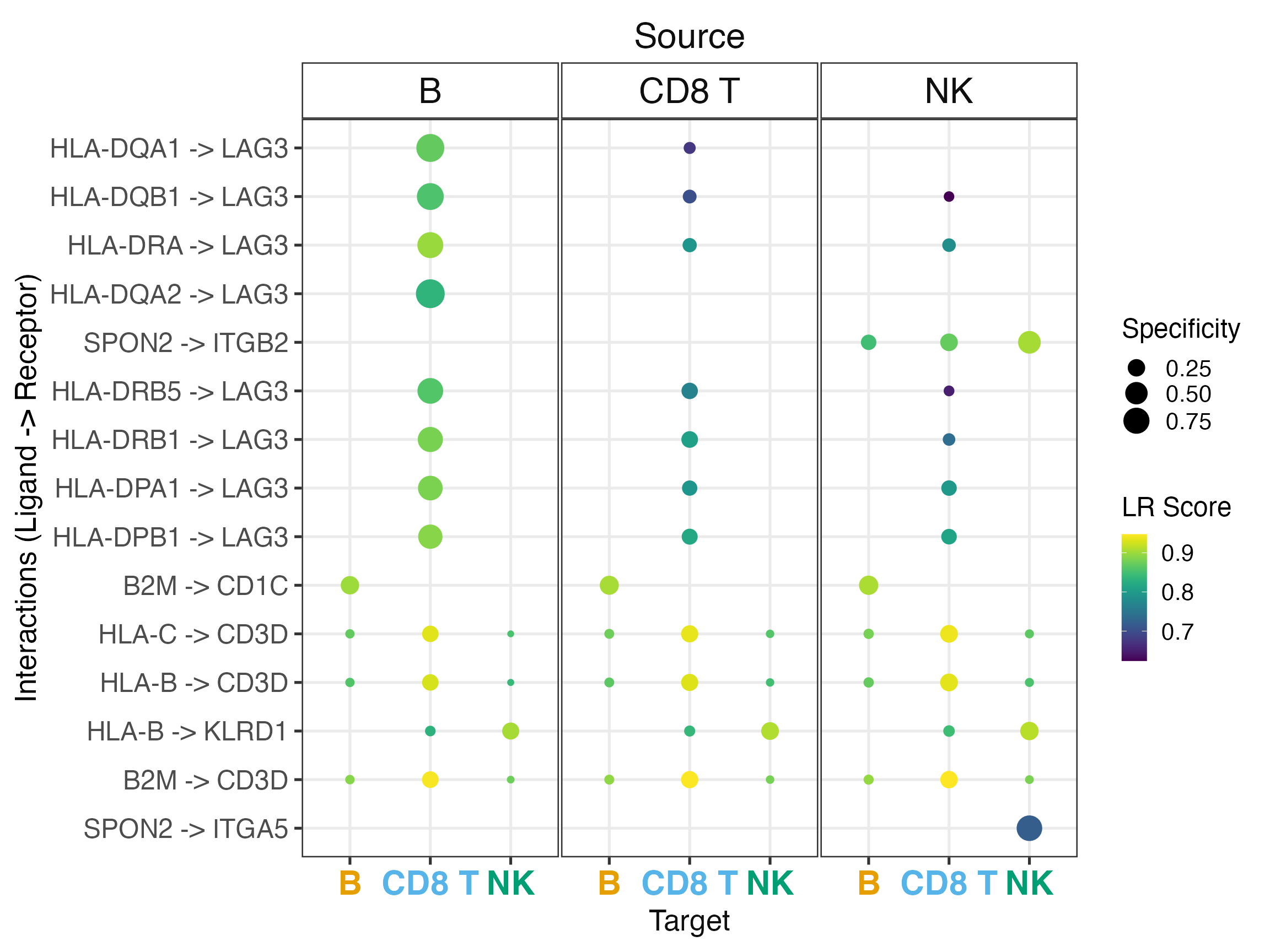
Custom Dotplot Parameters
# Use different metrics and adjust size
liana_aggr %>%
  liana_dotplot(
    ntop = 15,
    specificity = "natmi.edge_specificity",
    magnitude = "sca.LRscore",
    size_range = c(1, 8),
    size.label = "Specificity",
    colour.label = "LR Score"
  )
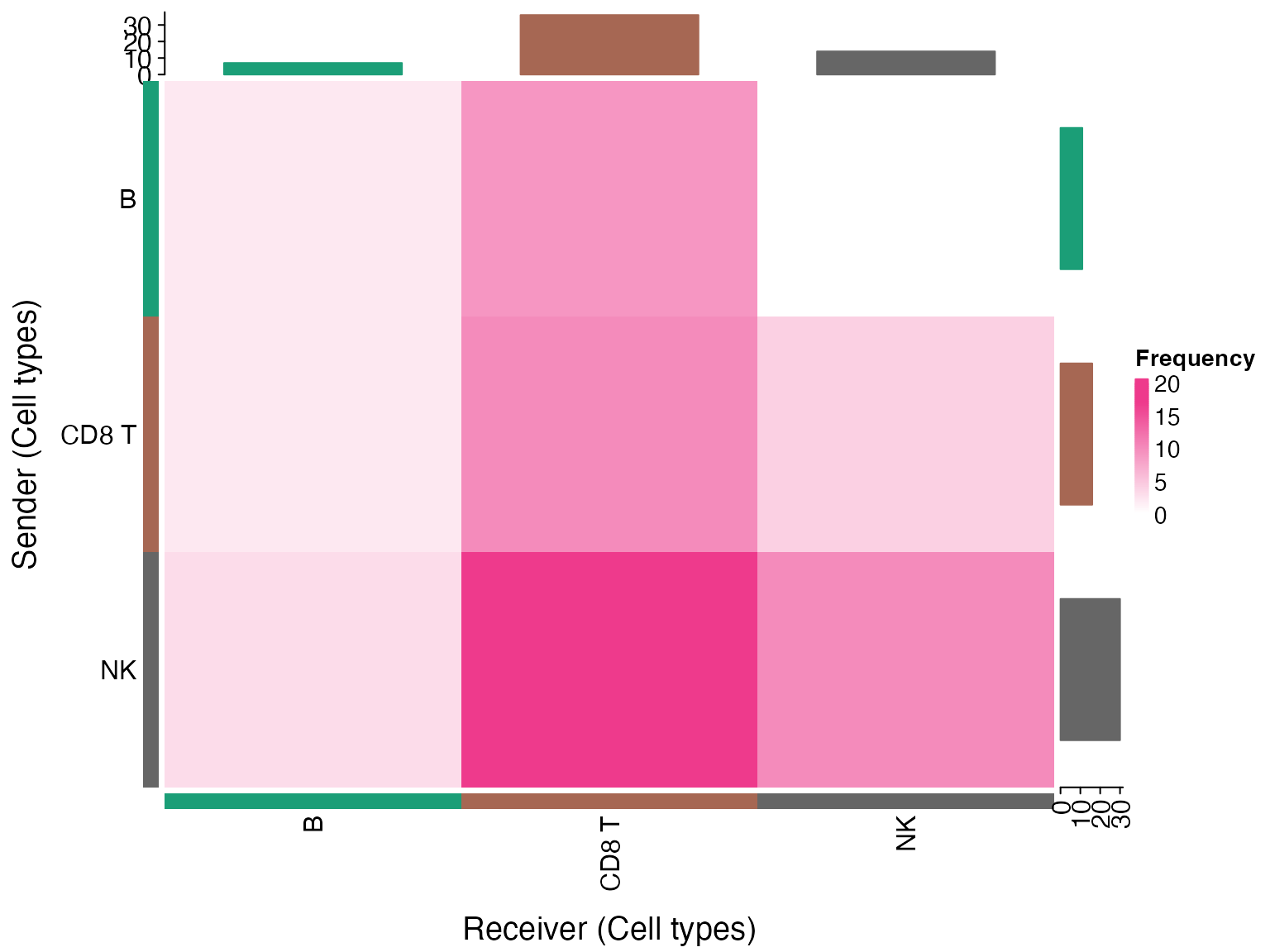
3. Chord Diagrams
Chord diagrams provide a circular visualization of cell-cell communication.
# Check if circlize is available
if(requireNamespace("circlize", quietly = TRUE) && nrow(liana_sig) > 0) {
  chord_freq(liana_sig)
}
Subset Chord Diagram
if(requireNamespace("circlize", quietly = TRUE) && nrow(liana_sig) > 0) {
  chord_freq(liana_sig,
    source_groups = c("CD8 T", "NK"),
    target_groups = c("CD8 T", "NK", "B"),
    cex = 1.2
  )
}
4. Custom ggplot2 Visualizations
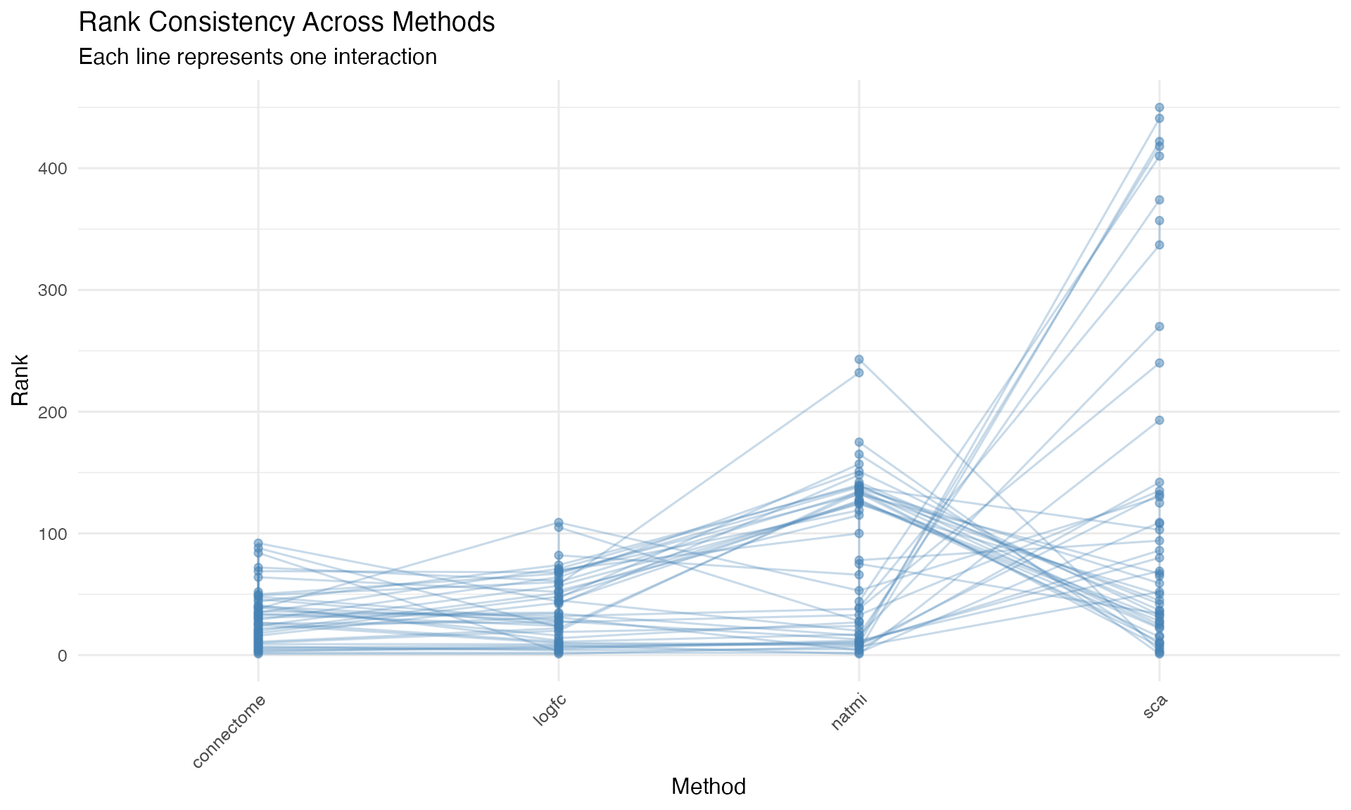
Method Comparison Plot
# Compare rankings across methods
liana_aggr %>%
  head(50) %>%
  select(ligand.complex, receptor.complex, source, target,
         ends_with(".rank")) %>%
  pivot_longer(cols = ends_with(".rank"),
               names_to = "method",
               values_to = "rank") %>%
  mutate(method = gsub("\\.rank", "", method)) %>%
  mutate(interaction = paste(ligand.complex, receptor.complex, sep = " -> ")) %>%
  ggplot(aes(x = method, y = rank, group = interaction)) +
  geom_line(alpha = 0.3, color = "steelblue") +
  geom_point(alpha = 0.5, color = "steelblue") +
  theme_minimal(base_size = 12) +
  theme(axis.text.x = element_text(angle = 45, hjust = 1)) +
  labs(
    title = "Rank Consistency Across Methods",
    subtitle = "Each line represents one interaction",
    x = "Method",
    y = "Rank"
  )
Score Distribution Plot
# Score distributions
liana_aggr %>%
  select(sca.LRscore, natmi.edge_specificity,
         connectome.weight_sc, logfc.logfc_comb) %>%
  pivot_longer(everything(), names_to = "Score", values_to = "Value") %>%
  ggplot(aes(x = Value, fill = Score)) +
  geom_density(alpha = 0.5) +
  facet_wrap(~Score, scales = "free") +
  theme_minimal(base_size = 11) +
  theme(legend.position = "none") +
  labs(title = "Distribution of LIANA Scores")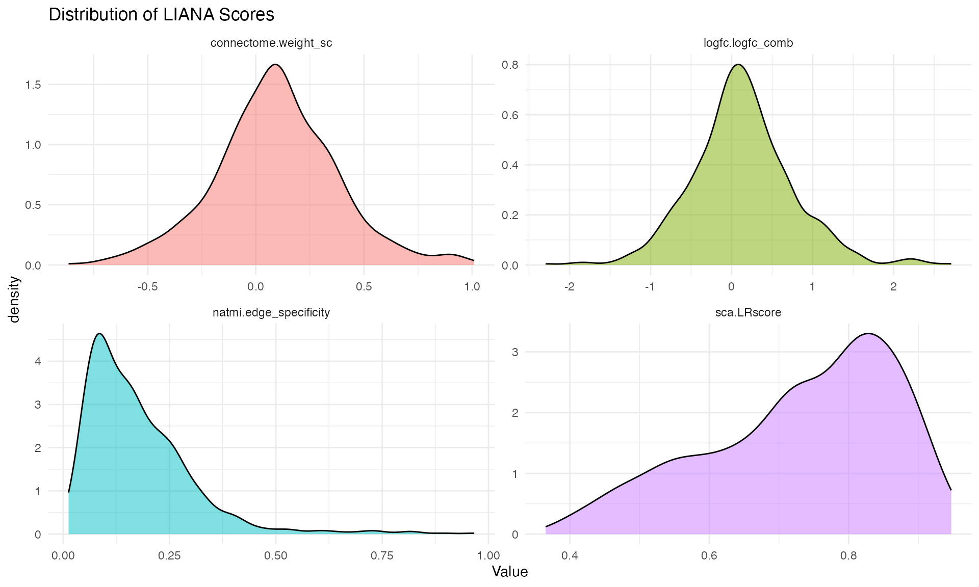
Top Interactions Bar Plot
liana_aggr %>%
  head(15) %>%
  mutate(interaction = paste(ligand.complex, "→", receptor.complex)) %>%
  mutate(cell_pair = paste(source, "→", target)) %>%
  ggplot(aes(x = reorder(interaction, -aggregate_rank),
             y = -log10(aggregate_rank + 1e-10),
             fill = cell_pair)) +
  geom_col() +
  coord_flip() +
  theme_minimal(base_size = 11) +
  labs(
    title = "Top 15 Cell-Cell Interactions",
    x = "Interaction (Ligand → Receptor)",
    y = "-log10(Aggregate Rank)",
    fill = "Cell Pair"
  ) +
  theme(legend.position = "right")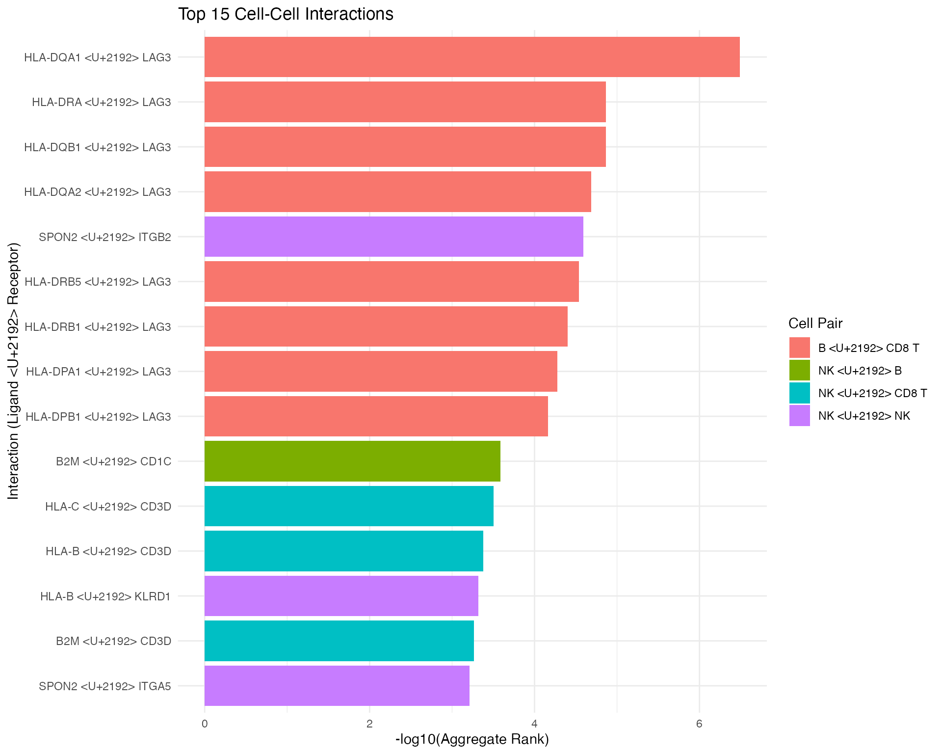
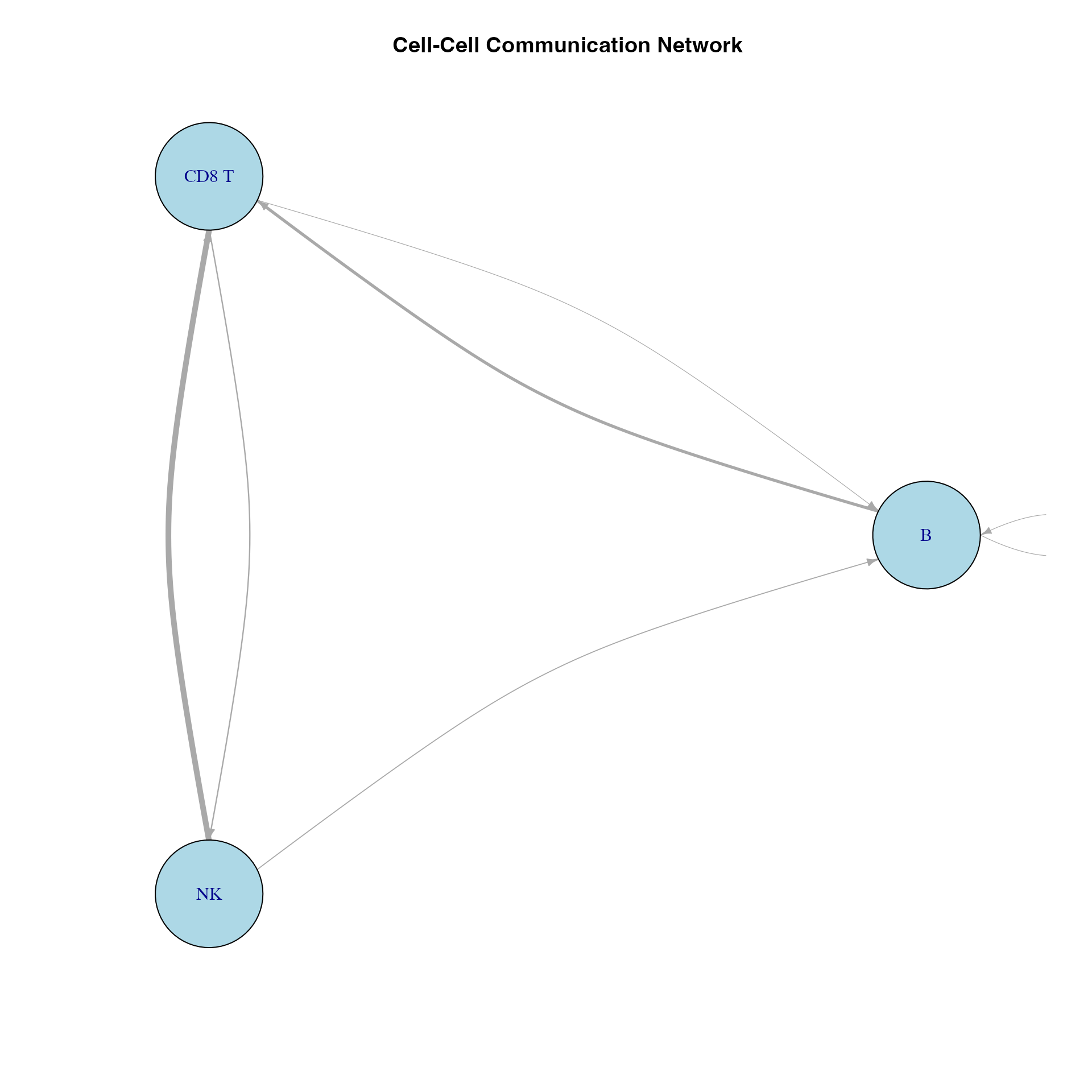
5. Network Visualization
Build Interaction Network
if(requireNamespace("igraph", quietly = TRUE) && nrow(liana_sig) > 0) {
  library(igraph)

  # Create edge list
  edges <- liana_sig %>%
    group_by(source, target) %>%
    summarise(weight = n(), .groups = "drop")

  # Create graph
  g <- graph_from_data_frame(edges, directed = TRUE)
  E(g)$width <- E(g)$weight / max(E(g)$weight) * 5

  # Plot
  plot(g,
    vertex.size = 30,
    vertex.label.cex = 1,
    vertex.color = "lightblue",
    edge.arrow.size = 0.5,
    edge.curved = 0.2,
    layout = layout_in_circle,
    main = "Cell-Cell Communication Network"
  )
}
6. Publication-Ready Figures
Combined Figure
library(patchwork)

# Create individual plots
p1 <- liana_aggr %>%
  head(10) %>%
  mutate(interaction = paste(ligand.complex, "→", receptor.complex)) %>%
  ggplot(aes(x = reorder(interaction, -aggregate_rank),
             y = sca.LRscore, fill = source)) +
  geom_col() +
  coord_flip() +
  theme_minimal() +
  labs(title = "A. Top Interactions by LRscore", x = "", y = "LR Score")

p2 <- liana_aggr %>%
  group_by(source, target) %>%
  summarise(n_int = sum(aggregate_rank <= 0.05), .groups = "drop") %>%
  ggplot(aes(x = source, y = target, fill = n_int)) +
  geom_tile() +
  scale_fill_viridis_c() +
  theme_minimal() +
  labs(title = "B. Significant Interactions per Cell Pair",
       fill = "Count", x = "Source", y = "Target")

p3 <- liana_aggr %>%
  ggplot(aes(x = sca.LRscore, y = natmi.edge_specificity,
             color = aggregate_rank <= 0.01)) +
  geom_point(alpha = 0.5) +
  scale_color_manual(values = c("gray70", "red"),
                     labels = c("NS", "Significant")) +
  theme_minimal() +
  labs(title = "C. Magnitude vs Specificity",
       x = "LR Score (Magnitude)",
       y = "Edge Specificity",
       color = "")

# Combine
(p1 | p2) / p3 +
  plot_annotation(title = "LIANA Cell-Cell Communication Analysis")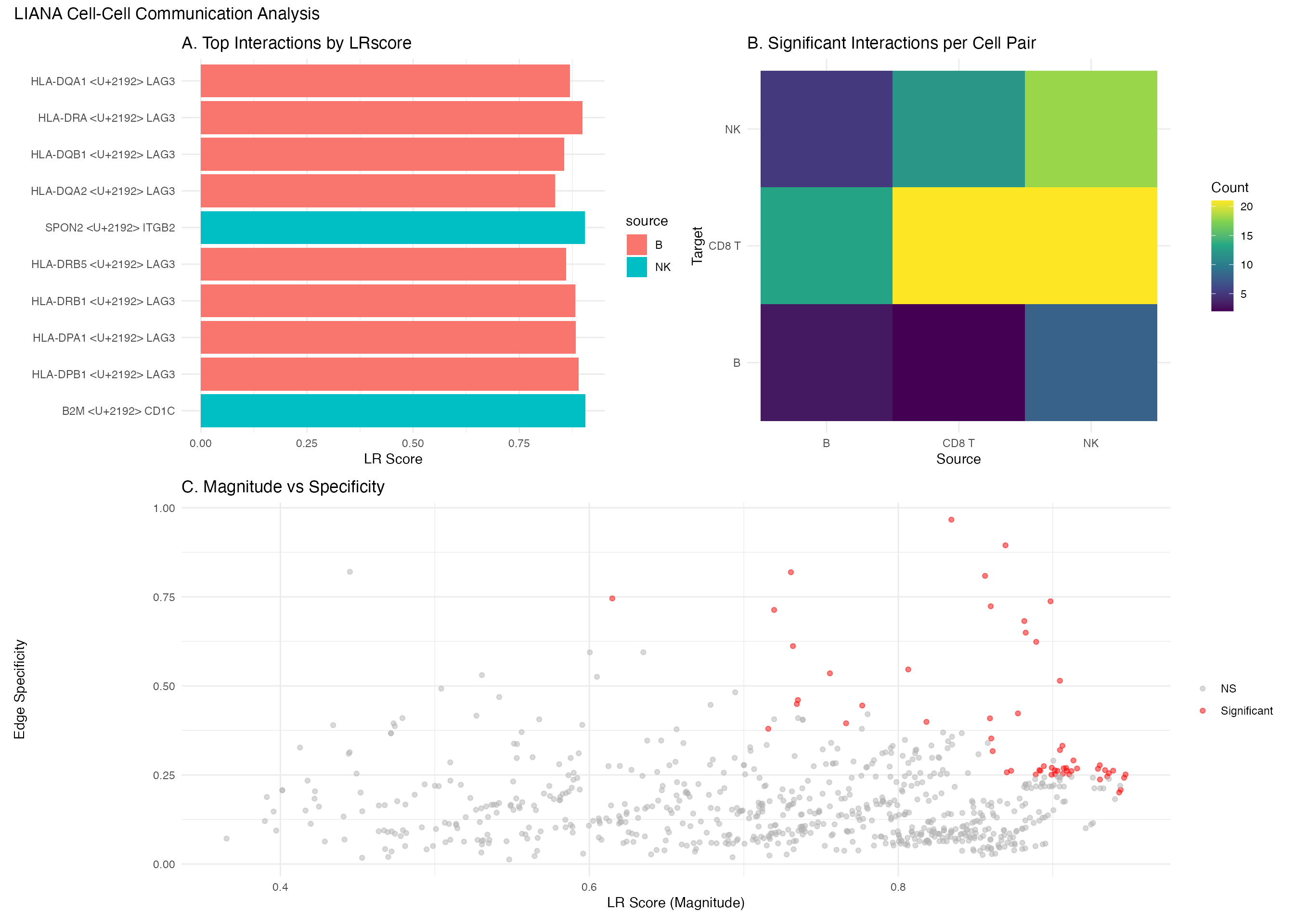
Tips for Effective Visualization
- Filter First: Always filter to significant interactions before plotting
-
Choose Appropriate Metrics:
- Magnitude for expression strength
- Specificity for cell-type exclusivity
-
Consider Your Audience:
- Dotplots for detailed inspection
- Heatmaps for overview
- Chord diagrams for presentations
- Export High Resolution:
ggsave("liana_figure.pdf", width = 12, height = 8, dpi = 300)Session Information
sessionInfo()
#> R version 4.4.0 (2024-04-24)
#> Platform: aarch64-apple-darwin20
#> Running under: macOS 15.6.1
#>
#> Matrix products: default
#> BLAS:   /Library/Frameworks/R.framework/Versions/4.4-arm64/Resources/lib/libRblas.0.dylib
#> LAPACK: /Library/Frameworks/R.framework/Versions/4.4-arm64/Resources/lib/libRlapack.dylib;  LAPACK version 3.12.0
#>
#> locale:
#> [1] C
#>
#> time zone: Asia/Shanghai
#> tzcode source: internal
#>
#> attached base packages:
#> [1] stats     graphics  grDevices utils     datasets  methods   base
#>
#> other attached packages:
#> [1] patchwork_1.3.2   igraph_2.2.1      tidyr_1.3.2       ggplot2_4.0.1
#> [5] dplyr_1.1.4       liana_0.1.14.9000 BiocStyle_2.34.0
#>
#> loaded via a namespace (and not attached):
#>   [1] spatstat.sparse_3.1-0       fs_1.6.6
#>   [3] matrixStats_1.5.0           lubridate_1.9.4
#>   [5] httr_1.4.7                  RColorBrewer_1.1-3
#>   [7] doParallel_1.0.17           tools_4.4.0
#>   [9] sctransform_0.4.3           backports_1.5.0
#>  [11] R6_2.6.1                    uwot_0.2.4
#>  [13] lazyeval_0.2.2              GetoptLong_1.1.0
#>  [15] withr_3.0.2                 sp_2.2-0
#>  [17] gridExtra_2.3               prettyunits_1.2.0
#>  [19] progressr_0.18.0            cli_3.6.5
#>  [21] Biobase_2.66.0              textshaping_1.0.4
#>  [23] Cairo_1.7-0                 spatstat.explore_3.6-0
#>  [25] labeling_0.4.3              sass_0.4.10
#>  [27] Seurat_4.4.0                spatstat.data_3.1-9
#>  [29] S7_0.2.1                    readr_2.1.6
#>  [31] ggridges_0.5.7              pbapply_1.7-4
#>  [33] pkgdown_2.1.3               systemfonts_1.3.1
#>  [35] R.utils_2.13.0              scater_1.34.1
#>  [37] dichromat_2.0-0.1           parallelly_1.46.1
#>  [39] sessioninfo_1.2.3           limma_3.62.2
#>  [41] readxl_1.4.5                RSQLite_2.4.5
#>  [43] generics_0.1.4              shape_1.4.6.1
#>  [45] spatstat.random_3.4-3       ica_1.0-3
#>  [47] zip_2.3.3                   Matrix_1.7-4
#>  [49] ggbeeswarm_0.7.3            S4Vectors_0.44.0
#>  [51] logger_0.4.1                abind_1.4-8
#>  [53] R.methodsS3_1.8.2           lifecycle_1.0.5
#>  [55] yaml_2.3.12                 edgeR_4.4.2
#>  [57] SummarizedExperiment_1.36.0 SparseArray_1.6.2
#>  [59] Rtsne_0.17                  grid_4.4.0
#>  [61] blob_1.2.4                  promises_1.5.0
#>  [63] dqrng_0.4.1                 crayon_1.5.3
#>  [65] dir.expiry_1.14.0           miniUI_0.1.2
#>  [67] lattice_0.22-7              beachmat_2.22.0
#>  [69] cowplot_1.2.0               chromote_0.5.1
#>  [71] magick_2.8.7                pillar_1.11.1
#>  [73] knitr_1.51                  ComplexHeatmap_2.22.0
#>  [75] metapod_1.14.0              GenomicRanges_1.58.0
#>  [77] tcltk_4.4.0                 rjson_0.2.23
#>  [79] future.apply_1.20.1         codetools_0.2-20
#>  [81] leiden_0.4.3.1              glue_1.8.0
#>  [83] spatstat.univar_3.1-6       data.table_1.18.0
#>  [85] vctrs_0.7.0                 png_0.1-8
#>  [87] cellranger_1.1.0            gtable_0.3.6
#>  [89] cachem_1.1.0                OmnipathR_3.19.1
#>  [91] xfun_0.56                   S4Arrays_1.6.0
#>  [93] mime_0.13                   survival_3.8-3
#>  [95] SingleCellExperiment_1.28.1 iterators_1.0.14
#>  [97] statmod_1.5.1               bluster_1.16.0
#>  [99] fitdistrplus_1.2-4          ROCR_1.0-11
#> [101] nlme_3.1-168                bit64_4.6.0-1
#> [103] progress_1.2.3              filelock_1.0.3
#> [105] RcppAnnoy_0.0.23            GenomeInfoDb_1.42.3
#> [107] bslib_0.9.0                 irlba_2.3.5.1
#> [109] vipor_0.4.7                 KernSmooth_2.23-26
#> [111] otel_0.2.0                  colorspace_2.1-2
#> [113] BiocGenerics_0.52.0         DBI_1.2.3
#> [115] tidyselect_1.2.1            processx_3.8.6
#> [117] bit_4.6.0                   compiler_4.4.0
#> [119] curl_7.0.0                  rvest_1.0.5
#> [121] httr2_1.2.2                 BiocNeighbors_2.0.1
#> [123] xml2_1.5.2                  desc_1.4.3
#> [125] DelayedArray_0.32.0         plotly_4.11.0
#> [127] bookdown_0.44               checkmate_2.3.3
#> [129] scales_1.4.0                lmtest_0.9-40
#> [131] rappdirs_0.3.4              goftest_1.2-3
#> [133] stringr_1.6.0               digest_0.6.39
#> [135] spatstat.utils_3.2-1        rmarkdown_2.30
#> [137] basilisk_1.23.0             XVector_0.46.0
#> [139] htmltools_0.5.9             pkgconfig_2.0.3
#> [141] sparseMatrixStats_1.18.0    MatrixGenerics_1.18.1
#> [143] fastmap_1.2.0               rlang_1.1.7
#> [145] GlobalOptions_0.1.3         htmlwidgets_1.6.4
#> [147] UCSC.utils_1.2.0            shiny_1.12.1
#> [149] farver_2.1.2                jquerylib_0.1.4
#> [151] zoo_1.8-15                  jsonlite_2.0.0
#> [153] BiocParallel_1.40.2         R.oo_1.27.1
#> [155] BiocSingular_1.22.0         magrittr_2.0.4
#> [157] scuttle_1.16.0              GenomeInfoDbData_1.2.13
#> [159] Rcpp_1.1.1                  viridis_0.6.5
#> [161] reticulate_1.44.1           stringi_1.8.7
#> [163] zlibbioc_1.52.0             MASS_7.3-65
#> [165] plyr_1.8.9                  parallel_4.4.0
#> [167] listenv_0.10.0              ggrepel_0.9.6
#> [169] deldir_2.0-4                splines_4.4.0
#> [171] tensor_1.5.1                hms_1.1.4
#> [173] circlize_0.4.17             locfit_1.5-9.12
#> [175] ps_1.9.1                    spatstat.geom_3.6-1
#> [177] reshape2_1.4.5              stats4_4.4.0
#> [179] ScaledMatrix_1.14.0         XML_3.99-0.20
#> [181] evaluate_1.0.5              SeuratObject_4.1.4
#> [183] scran_1.34.0                BiocManager_1.30.27
#> [185] tzdb_0.5.0                  foreach_1.5.2
#> [187] httpuv_1.6.16               polyclip_1.10-7
#> [189] RANN_2.6.2                  purrr_1.2.1
#> [191] future_1.69.0               clue_0.3-66
#> [193] scattermore_1.2             rsvd_1.0.5
#> [195] xtable_1.8-4                later_1.4.5
#> [197] viridisLite_0.4.2           ragg_1.5.0
#> [199] tibble_3.3.1                websocket_1.4.4
#> [201] beeswarm_0.4.0              memoise_2.0.1
#> [203] IRanges_2.40.1              cluster_2.1.8.1
#> [205] timechange_0.3.0            globals_0.18.0