Introduction
CytoSPACER provides comprehensive visualization functions built on
ggplot2. This vignette showcases the various plotting
options available for exploring and presenting your results.
Generate Example Data
First, let’s create a simulated dataset:
set.seed(123)

# Parameters
n_genes <- 100
n_cells <- 500
n_spots <- 50

# Create scRNA-seq data
sc_data <- matrix(rpois(n_genes * n_cells, lambda = 5), nrow = n_genes, ncol = n_cells)
rownames(sc_data) <- paste0("Gene", seq_len(n_genes))
colnames(sc_data) <- paste0("Cell", seq_len(n_cells))

# Define cell types
cell_types <- rep(c("TypeA", "TypeB", "TypeC", "TypeD", "TypeE"), each = 100)
names(cell_types) <- colnames(sc_data)

# Add cell type-specific expression
for (i in 1:5) {
  marker_genes <- ((i-1)*20 + 1):(i*20)
  type_cells <- which(cell_types == unique(cell_types)[i])
  sc_data[marker_genes, type_cells] <- sc_data[marker_genes, type_cells] + 20
}

# Create ST data
st_data <- matrix(rpois(n_genes * n_spots, lambda = 50), nrow = n_genes, ncol = n_spots)
rownames(st_data) <- paste0("Gene", seq_len(n_genes))
colnames(st_data) <- paste0("Spot", seq_len(n_spots))

# Create spatial coordinates (grid pattern)
coordinates <- data.frame(
  row = rep(1:10, each = 5),
  col = rep(1:5, times = 10),
  row.names = colnames(st_data)
)

# Create cell type fractions
unique_types <- unique(cell_types)
n_types <- length(unique_types)
cell_type_fractions <- as.data.frame(matrix(
  1/n_types, nrow = n_spots, ncol = n_types,
  dimnames = list(colnames(st_data), unique_types)
))

# Run CytoSPACER
results <- run_cytospace(
  sc_data = sc_data,
  cell_types = cell_types,
  st_data = st_data,
  coordinates = coordinates,
  cell_type_fractions = cell_type_fractions,
  mean_cells_per_spot = 5,
  seed = 42,
  verbose = FALSE
)
Basic Spatial Plots
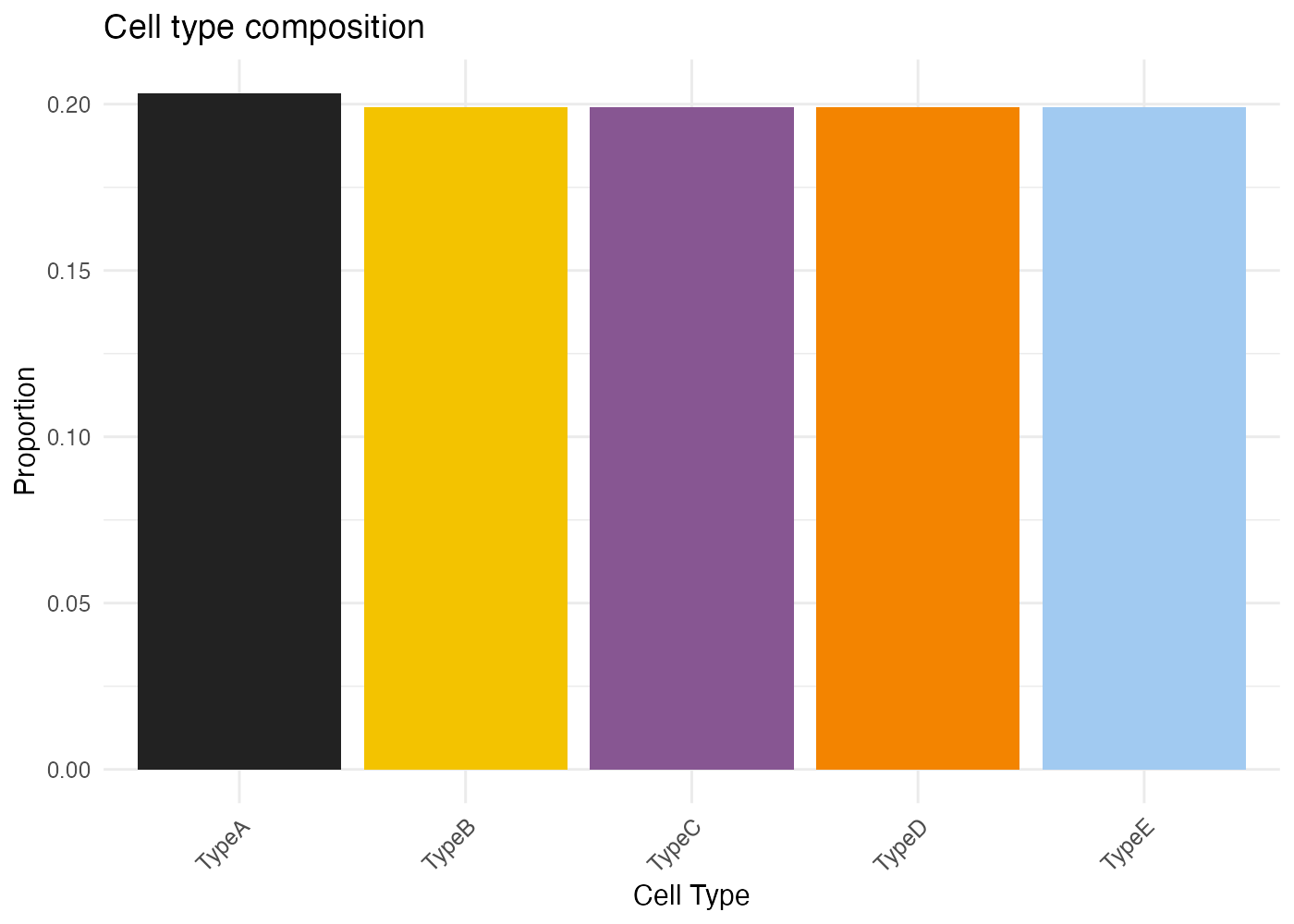
Cell Type Distribution
The primary visualization shows the spatial distribution of assigned cell types:
plot_cytospace(results, type = "cell_types")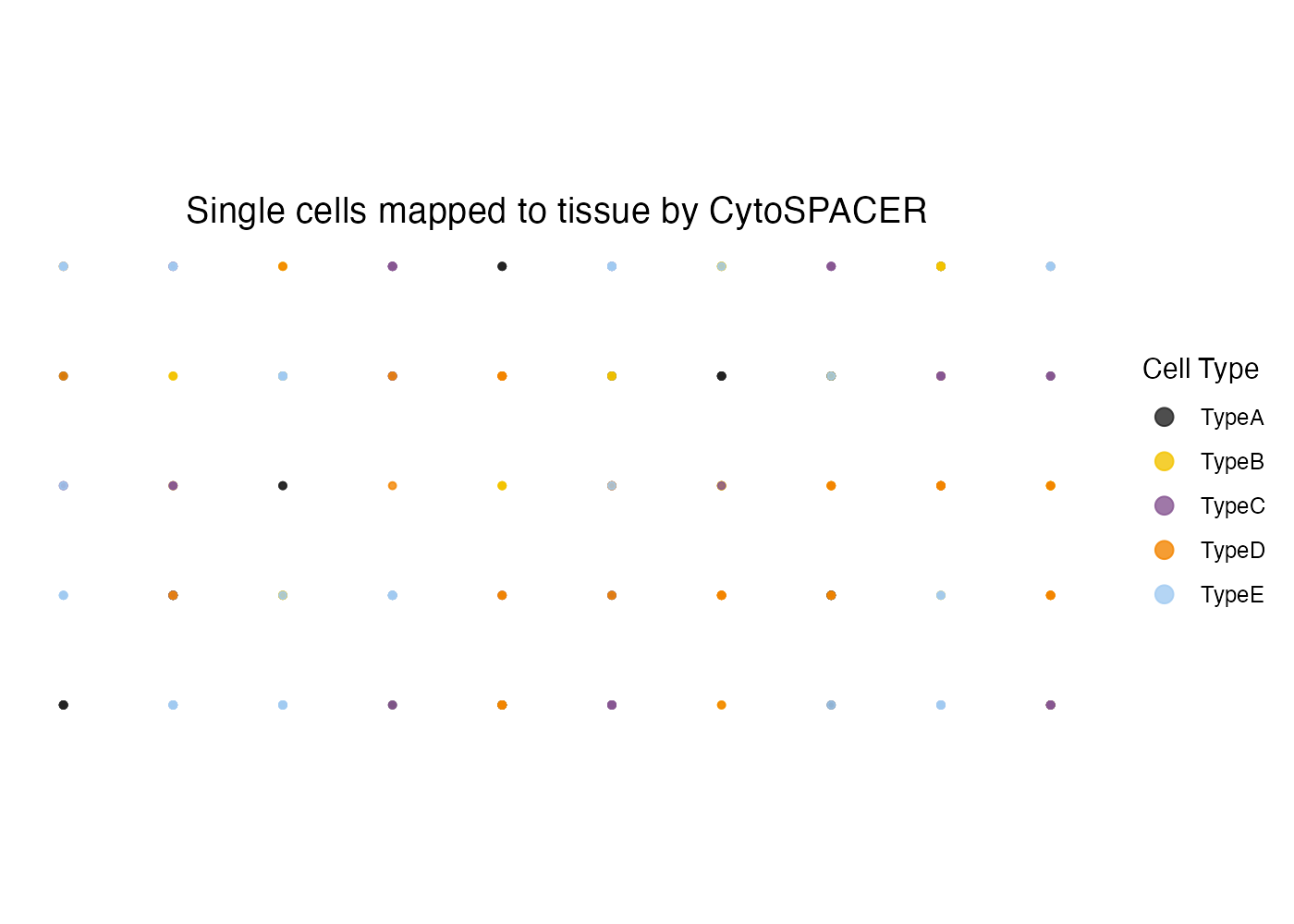
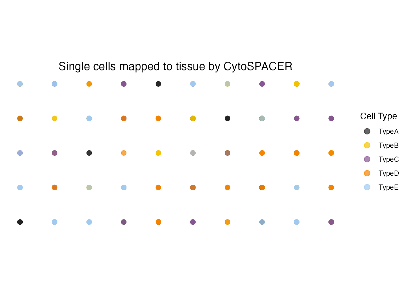
Customizing Point Size and Transparency
plot_cytospace(
  results,
  type = "cell_types",
  point_size = 2.5,
  alpha = 0.7
)
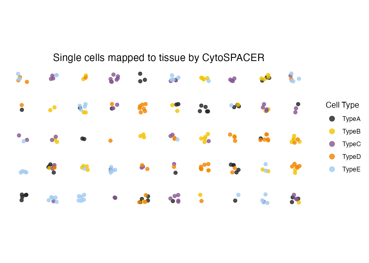
Adding Jitter
For dense regions where points overlap, add jitter:
plot_cytospace(
  results,
  type = "cell_types",
  jitter = 0.3,
  point_size = 2
)
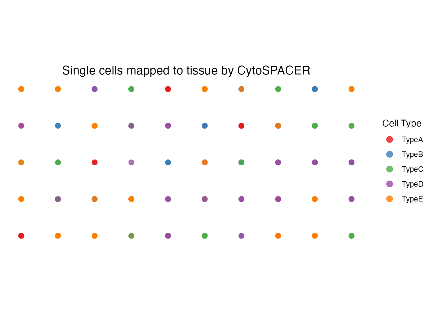
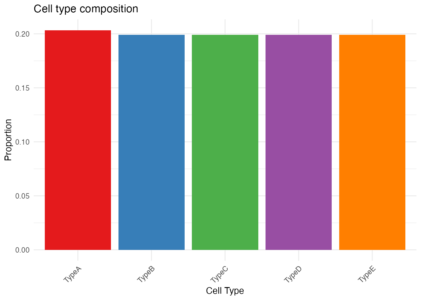
Custom Colors
my_colors <- c(
  "TypeA" = "#E41A1C",
  "TypeB" = "#377EB8",
  "TypeC" = "#4DAF4A",
  "TypeD" = "#984EA3",
  "TypeE" = "#FF7F00"
)

plot_cytospace(
  results,
  type = "cell_types",
  colors = my_colors,
  point_size = 2.5
)
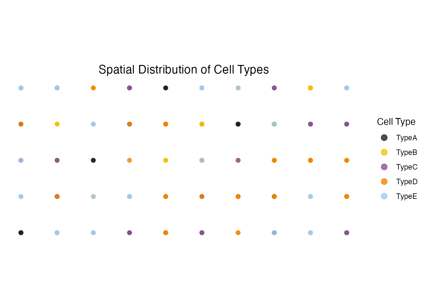
Custom Title
plot_cytospace(
  results,
  type = "cell_types",
  title = "Spatial Distribution of Cell Types",
  point_size = 2
)
Advanced Visualizations
Combining with ggplot2
Since all plots are ggplot2 objects, you can easily customize them:
p <- plot_cytospace(results, type = "cell_types", colors = my_colors)

# Add custom theme
p +
  theme_minimal() +
  theme(
    legend.position = "bottom",
    legend.title = element_text(face = "bold"),
    plot.title = element_text(hjust = 0.5, size = 16, face = "bold")
  ) +
  guides(color = guide_legend(nrow = 1, override.aes = list(size = 4)))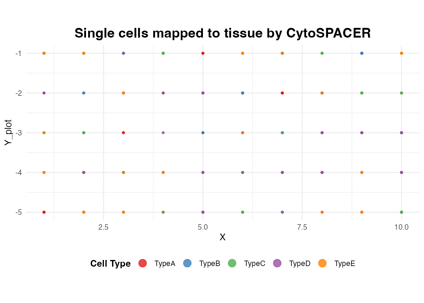
Faceted by Cell Type
# Get the assigned locations data
locs <- results$assigned_locations
locs$Y_plot <- -locs$col

# Create faceted plot
ggplot(locs, aes(x = row, y = Y_plot)) +
  geom_point(aes(color = CellType), size = 1.5, alpha = 0.8) +
  facet_wrap(~ CellType, ncol = 3) +
  scale_color_manual(values = my_colors) +
  coord_equal() +
  theme_minimal() +
  theme(
    axis.text = element_blank(),
    axis.title = element_blank(),
    axis.ticks = element_blank(),
    panel.grid = element_blank(),
    strip.text = element_text(face = "bold", size = 11),
    legend.position = "none"
  ) +
  labs(title = "Cell Type Distribution by Type")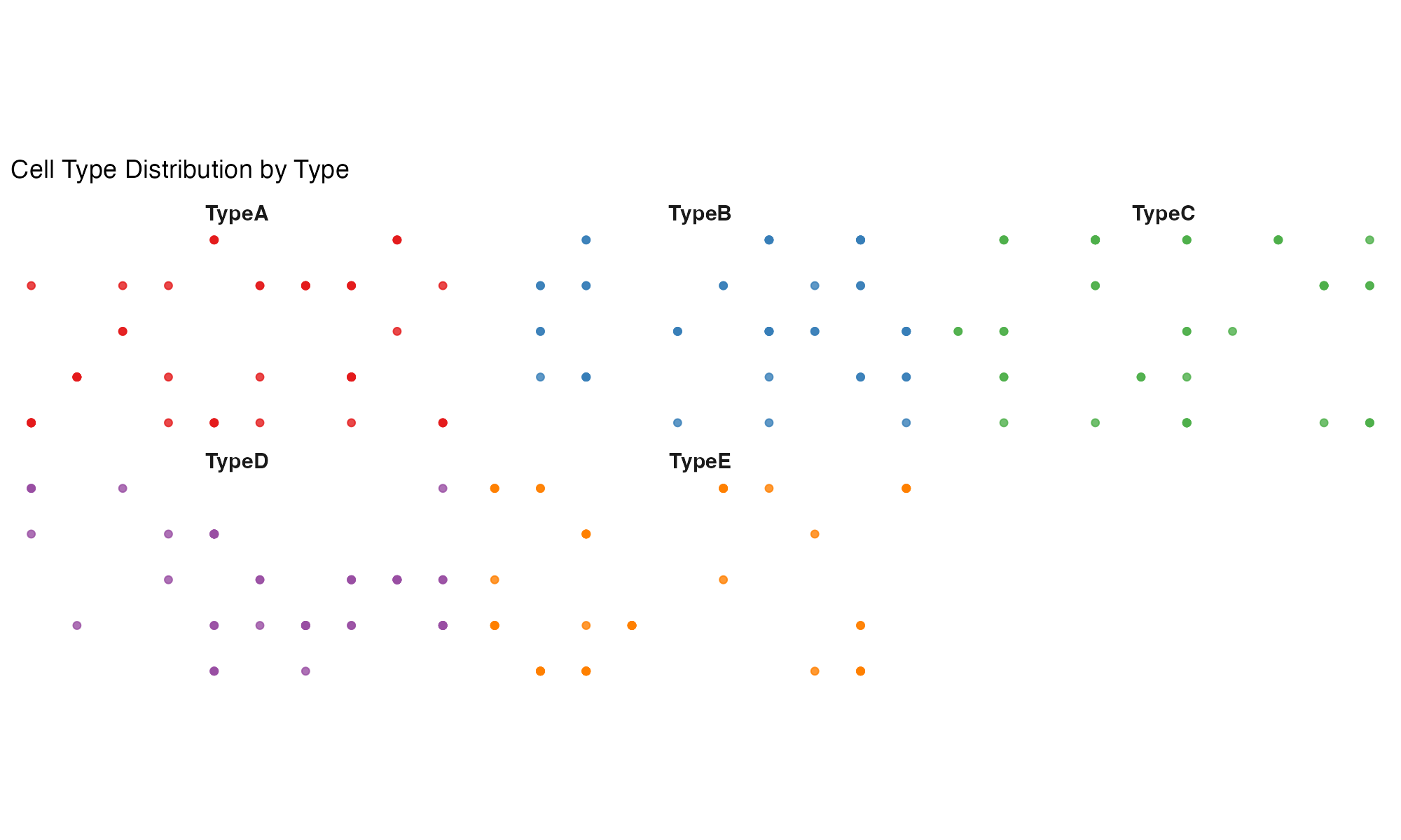
Saving Plots
# Save individual plot
p <- plot_cytospace(results, type = "cell_types", colors = my_colors)

# Using CytoSPACER function
save_cytospace_plot(
  plot = p,
  output_dir = "figures/",
  prefix = "spatial_",
  formats = c("png", "pdf"),
  width = 10,
  height = 8,
  dpi = 300
)

# Using ggplot2 directly
ggsave("figures/cell_types.png", p, width = 10, height = 8, dpi = 300)
Color Palettes
CytoSPACER includes a built-in color palette optimized for distinguishing cell types:
# Default CytoSPACER colors (first 10)
default_colors <- c(
  "#222222", "#F3C300", "#875692", "#F38400", "#A1CAF1",
  "#BE0032", "#C2B280", "#848482", "#008856", "#E68FAC"
)

# Display palette
barplot(rep(1, 10), col = default_colors, border = NA, axes = FALSE,
        main = "CytoSPACER Default Color Palette", names.arg = 1:10)
Session Info
sessionInfo()
#> R version 4.4.0 (2024-04-24)
#> Platform: aarch64-apple-darwin20
#> Running under: macOS 15.6.1
#>
#> Matrix products: default
#> BLAS:   /Library/Frameworks/R.framework/Versions/4.4-arm64/Resources/lib/libRblas.0.dylib
#> LAPACK: /Library/Frameworks/R.framework/Versions/4.4-arm64/Resources/lib/libRlapack.dylib;  LAPACK version 3.12.0
#>
#> locale:
#> [1] C
#>
#> time zone: Asia/Shanghai
#> tzcode source: internal
#>
#> attached base packages:
#> [1] stats     graphics  grDevices utils     datasets  methods   base
#>
#> other attached packages:
#> [1] ggplot2_4.0.1    CytoSPACER_1.0.0
#>
#> loaded via a namespace (and not attached):
#>  [1] sass_0.4.10         future_1.69.0       generics_0.1.4
#>  [4] lattice_0.22-7      listenv_0.10.0      digest_0.6.39
#>  [7] magrittr_2.0.4      evaluate_1.0.5      grid_4.4.0
#> [10] RColorBrewer_1.1-3  fastmap_1.2.0       jsonlite_2.0.0
#> [13] Matrix_1.7-4        scales_1.4.0        codetools_0.2-20
#> [16] textshaping_1.0.4   jquerylib_0.1.4     cli_3.6.5
#> [19] rlang_1.1.7         parallelly_1.46.1   future.apply_1.20.1
#> [22] withr_3.0.2         cachem_1.1.0        yaml_2.3.12
#> [25] otel_0.2.0          tools_4.4.0         parallel_4.4.0
#> [28] dplyr_1.1.4         globals_0.18.0      vctrs_0.7.1
#> [31] R6_2.6.1            lifecycle_1.0.5     fs_1.6.6
#> [34] htmlwidgets_1.6.4   ragg_1.5.0          pkgconfig_2.0.3
#> [37] desc_1.4.3          pkgdown_2.1.3       progressr_0.18.0
#> [40] bslib_0.9.0         pillar_1.11.1       gtable_0.3.6
#> [43] data.table_1.18.0   glue_1.8.0          Rcpp_1.1.1
#> [46] systemfonts_1.3.1   xfun_0.56           tibble_3.3.1
#> [49] tidyselect_1.2.1    knitr_1.51          dichromat_2.0-0.1
#> [52] farver_2.1.2        htmltools_0.5.9     rmarkdown_2.30
#> [55] labeling_0.4.3      compiler_4.4.0      S7_0.2.1