Introduction
CytoSPACER is an R implementation of CytoSPACE (Vahid et al., Nature Biotechnology, 2023), designed for high-resolution mapping of single-cell transcriptomes to spatial transcriptomics (ST) data. This vignette provides a quick introduction to get you started with the package.
Installation
# From R-universe (recommended)
install.packages("CytoSPACER", repos = "https://zaoqu-liu.r-universe.dev")

# From GitHub
remotes::install_github("Zaoqu-Liu/CytoSPACER")Simulated Example
Let’s create a simple simulated dataset to demonstrate the workflow:
set.seed(42)

# Simulate scRNA-seq data (100 genes x 500 cells)
n_genes <- 100
n_cells <- 500
n_spots <- 50

# Create expression matrix with some structure
sc_data <- matrix(
  rpois(n_genes * n_cells, lambda = 5),
  nrow = n_genes,
  ncol = n_cells
)
rownames(sc_data) <- paste0("Gene", seq_len(n_genes))
colnames(sc_data) <- paste0("Cell", seq_len(n_cells))

# Add cell type-specific expression patterns
cell_types <- rep(c("TypeA", "TypeB", "TypeC", "TypeD", "TypeE"), each = 100)
names(cell_types) <- colnames(sc_data)

# TypeA cells express genes 1-20 highly
sc_data[1:20, cell_types == "TypeA"] <- sc_data[1:20, cell_types == "TypeA"] + 20
# TypeB cells express genes 21-40 highly
sc_data[21:40, cell_types == "TypeB"] <- sc_data[21:40, cell_types == "TypeB"] + 20
# TypeC cells express genes 41-60 highly
sc_data[41:60, cell_types == "TypeC"] <- sc_data[41:60, cell_types == "TypeC"] + 20

# Simulate ST data (100 genes x 50 spots)
st_data <- matrix(
  rpois(n_genes * n_spots, lambda = 50),
  nrow = n_genes,
  ncol = n_spots
)
rownames(st_data) <- paste0("Gene", seq_len(n_genes))
colnames(st_data) <- paste0("Spot", seq_len(n_spots))

# Create spatial coordinates (grid pattern)
coordinates <- data.frame(
  row = rep(1:10, each = 5),
  col = rep(1:5, times = 10),
  row.names = colnames(st_data)
)

# Display data dimensions
cat("scRNA-seq data:", nrow(sc_data), "genes x", ncol(sc_data), "cells\n")
#> scRNA-seq data: 100 genes x 500 cells
cat("ST data:", nrow(st_data), "genes x", ncol(st_data), "spots\n")
#> ST data: 100 genes x 50 spots
cat("Cell types:", paste(unique(cell_types), collapse = ", "), "\n")
#> Cell types: TypeA, TypeB, TypeC, TypeD, TypeE
Run CytoSPACER
Now let’s run the main analysis. We’ll provide pre-computed cell type fractions to skip the Seurat-dependent deconvolution step:
# Create simple cell type fractions (for demonstration)
# In real analysis, these would be estimated from the data
unique_types <- unique(cell_types)
n_types <- length(unique_types)
cell_type_fractions <- matrix(
  1/n_types,
  nrow = n_spots,
  ncol = n_types,
  dimnames = list(colnames(st_data), unique_types)
)
cell_type_fractions <- as.data.frame(cell_type_fractions)

# Run CytoSPACER with default parameters
results <- run_cytospace(
  sc_data = sc_data,
  cell_types = cell_types,
  st_data = st_data,
  coordinates = coordinates,
  cell_type_fractions = cell_type_fractions,
  mean_cells_per_spot = 5,
  distance_metric = "pearson",
  sampling_method = "duplicates",
  seed = 42,
  verbose = TRUE
)
Explore Results
The results object contains several components:
# Check the structure
names(results)
#> [1] "assigned_locations"    "expression"            "cell_type_by_spot"
#> [4] "fractional_abundances" "parameters"            "log"
#> [7] "runtime"

# View assigned locations
head(results$assigned_locations)
#>   UniqueCID OriginalCID CellType SpotID row col
#> 1   UCID001      Cell49    TypeA Spot26   6   1
#> 2   UCID002      Cell65    TypeA Spot28   6   3
#> 3   UCID003      Cell25    TypeA Spot26   6   1
#> 4   UCID004      Cell74    TypeA Spot28   6   3
#> 5   UCID005      Cell18    TypeA Spot26   6   1
#> 6   UCID006     Cell100    TypeA Spot28   6   3

# Cell type counts per spot
head(results$cell_type_by_spot)
#>        TypeA TypeB TypeC TypeD TypeE Total
#> Spot1      0     0     0     4     0     4
#> Spot10     0     2     0     1     0     3
#> Spot11     1     1     3     0     2     7
#> Spot12     2     0     1     0     0     3
#> Spot13     0     0     0     1     2     3
#> Spot14     6     0     0     0     0     6

# Fractional abundances
head(results$fractional_abundances)
#>            TypeA     TypeB     TypeC     TypeD     TypeE
#> Spot1  0.0000000 0.0000000 0.0000000 1.0000000 0.0000000
#> Spot10 0.0000000 0.6666667 0.0000000 0.3333333 0.0000000
#> Spot11 0.1428571 0.1428571 0.4285714 0.0000000 0.2857143
#> Spot12 0.6666667 0.0000000 0.3333333 0.0000000 0.0000000
#> Spot13 0.0000000 0.0000000 0.0000000 0.3333333 0.6666667
#> Spot14 1.0000000 0.0000000 0.0000000 0.0000000 0.0000000
Visualization
CytoSPACER provides several visualization functions:
Spatial Cell Type Distribution
# Plot cell type spatial distribution
plot_cytospace(results, type = "cell_types", point_size = 2)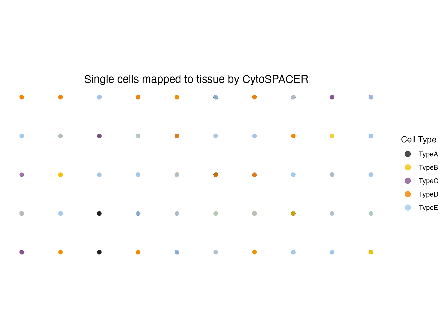
With Jitter for Dense Regions
# Add jitter to separate overlapping points
plot_cytospace(results, type = "cell_types", jitter = 0.3, point_size = 2)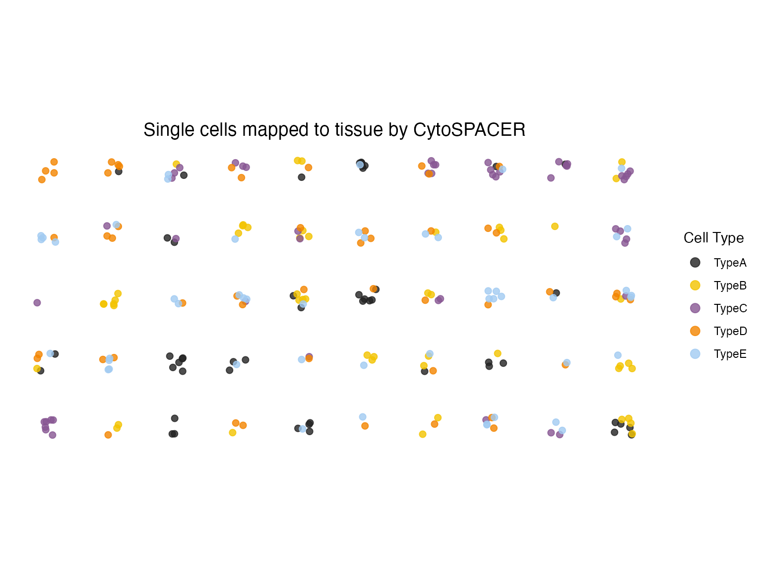
Summary Statistics
# Total cells assigned
cat("Total cells assigned:", nrow(results$assigned_locations), "\n")
#> Total cells assigned: 249
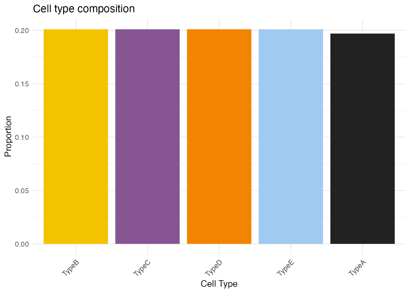
# Cells per cell type
table(results$assigned_locations$CellType)
#>
#> TypeA TypeB TypeC TypeD TypeE
#> 49 50 50 50 50
# Average cells per spot
cat("Average cells per spot:",
mean(results$cell_type_by_spot$Total), "\n")
#> Average cells per spot: 4.98
# Runtime
cat("Analysis runtime:", round(results$runtime, 2), "seconds\n")
#> Analysis runtime: 0.04 secondsSave Results
# Save results to files
write_cytospace_results(results, output_dir = "cytospace_output/")
Next Steps
- See the Algorithm Principles vignette for detailed methodology
- See the Visualization Gallery for more plotting options
- See the Seurat Integration for working with Seurat objects
- See the Performance Optimization for large datasets
Session Info
sessionInfo()
#> R version 4.4.0 (2024-04-24)
#> Platform: aarch64-apple-darwin20
#> Running under: macOS 15.6.1
#>
#> Matrix products: default
#> BLAS:   /Library/Frameworks/R.framework/Versions/4.4-arm64/Resources/lib/libRblas.0.dylib
#> LAPACK: /Library/Frameworks/R.framework/Versions/4.4-arm64/Resources/lib/libRlapack.dylib;  LAPACK version 3.12.0
#>
#> locale:
#> [1] C
#>
#> time zone: Asia/Shanghai
#> tzcode source: internal
#>
#> attached base packages:
#> [1] stats     graphics  grDevices utils     datasets  methods   base
#>
#> other attached packages:
#> [1] CytoSPACER_1.0.0
#>
#> loaded via a namespace (and not attached):
#>  [1] sass_0.4.10         future_1.69.0       generics_0.1.4
#>  [4] lattice_0.22-7      listenv_0.10.0      digest_0.6.39
#>  [7] magrittr_2.0.4      evaluate_1.0.5      grid_4.4.0
#> [10] RColorBrewer_1.1-3  fastmap_1.2.0       jsonlite_2.0.0
#> [13] Matrix_1.7-4        scales_1.4.0        codetools_0.2-20
#> [16] textshaping_1.0.4   jquerylib_0.1.4     cli_3.6.5
#> [19] rlang_1.1.7         parallelly_1.46.1   future.apply_1.20.1
#> [22] withr_3.0.2         cachem_1.1.0        yaml_2.3.12
#> [25] otel_0.2.0          tools_4.4.0         parallel_4.4.0
#> [28] dplyr_1.1.4         ggplot2_4.0.1       globals_0.18.0
#> [31] vctrs_0.7.1         R6_2.6.1            lifecycle_1.0.5
#> [34] fs_1.6.6            htmlwidgets_1.6.4   ragg_1.5.0
#> [37] pkgconfig_2.0.3     desc_1.4.3          pkgdown_2.1.3
#> [40] progressr_0.18.0    bslib_0.9.0         pillar_1.11.1
#> [43] gtable_0.3.6        data.table_1.18.0   glue_1.8.0
#> [46] Rcpp_1.1.1          systemfonts_1.3.1   xfun_0.56
#> [49] tibble_3.3.1        tidyselect_1.2.1    knitr_1.51
#> [52] dichromat_2.0-0.1   farver_2.1.2        htmltools_0.5.9
#> [55] rmarkdown_2.30      labeling_0.4.3      compiler_4.4.0
#> [58] S7_0.2.1