MAGIC Algorithm: Mathematical Foundations

Introduction

This vignette provides a comprehensive mathematical description of the MAGIC algorithm. Understanding these foundations helps users make informed decisions about parameter selection and interpret results correctly.

The Dropout Problem in scRNA-seq

Single-cell RNA sequencing captures transcriptomic profiles at single-cell resolution, but suffers from technical limitations:

Low capture efficiency: Only 10-20% of mRNA molecules are captured
Amplification bias: PCR amplification introduces noise
Dropout events: Expressed genes appear as zeros due to sampling

These issues result in sparse, noisy count matrices where biological signal is obscured.

MAGIC: A Diffusion-Based Solution

MAGIC leverages the manifold hypothesis: high-dimensional single-cell data lies on a lower-dimensional manifold reflecting biological states. By diffusing information along this manifold, MAGIC recovers missing transcripts while preserving biological structure.

Algorithm Steps

Step 1: Dimensionality Reduction (Optional)

For computational efficiency, MAGIC first reduces dimensionality using PCA:

$X_{pca} = X \cdot V_k$

where $V_k$ contains the top $k$ principal components (default: 100).

Step 2: k-Nearest Neighbor Graph

For each cell $i$ , identify its $k$ nearest neighbors based on Euclidean distance in PCA space:

$\mathcal{N}_k(i) = \{j : d(x_i, x_j) \leq d_k(x_i)\}$

where $d_k(x_i)$ is the distance to the $k$ -th nearest neighbor.

Step 3: α-Decaying Kernel

The affinity between cells is computed using an α-decaying kernel with adaptive bandwidth:

$K(x_i, x_j) = \exp\left(-\left(\frac{\|x_i - x_j\|_2}{\varepsilon_i}\right)^\alpha\right)$

where:

$\varepsilon_i = d_k(x_i)$ is the adaptive bandwidth (distance to $k$ -th neighbor)
$\alpha$ controls kernel sharpness (default: 1)

Why adaptive bandwidth?

Accounts for varying local density
Cells in dense regions have smaller bandwidth
Cells in sparse regions have larger bandwidth
Preserves rare cell populations

# Visualize α-decaying kernel
x <- seq(0, 3, length.out = 100)

par(mfrow = c(1, 2))

# Effect of distance
plot(x, exp(-x), type = "l", lwd = 2, col = "#e74c3c",
     xlab = "Normalized Distance (d/ε)", ylab = "Affinity K(x,y)",
     main = "α-Decaying Kernel (α = 1)")
abline(h = 0.5, lty = 2, col = "gray")
abline(v = log(2), lty = 2, col = "gray")

# Effect of α
plot(x, exp(-x^0.5), type = "l", lwd = 2, col = "#3498db",
     xlab = "Normalized Distance (d/ε)", ylab = "Affinity K(x,y)",
     main = "Effect of α Parameter", ylim = c(0, 1))
lines(x, exp(-x^1), lwd = 2, col = "#e74c3c")
lines(x, exp(-x^2), lwd = 2, col = "#2ecc71")
legend("topright", legend = c("α = 0.5", "α = 1", "α = 2"),
       col = c("#3498db", "#e74c3c", "#2ecc71"), lwd = 2)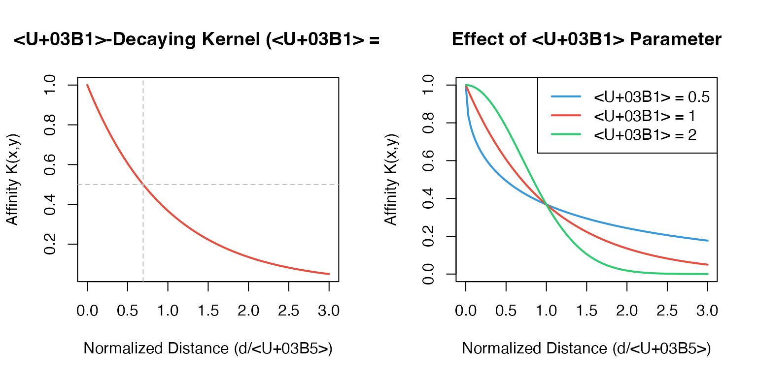

Step 4: Markov Normalization

The kernel matrix is row-normalized to create a Markov transition matrix:

$P = D^{-1}K$

where $D$ is the diagonal degree matrix with $D_{ii} = \sum_j K_{ij}$ .

Properties of P:

Row-stochastic: $\sum_j P_{ij} = 1$
Represents transition probabilities in a random walk
Eigenvalues in $[-1, 1]$

Step 5: Diffusion (Powering)

The diffusion operator is powered $t$ times:

$X_{imputed} = P^t X$

Each power of $P$ propagates information one step along the graph:

$t = 1$ : Local averaging with immediate neighbors
$t = 2$ : Information from 2-hop neighbors
$t = t$ : Information from $t$ -hop neighborhood

# Simulate diffusion effect
set.seed(42)
n <- 100
x <- c(rnorm(50, -2, 0.5), rnorm(50, 2, 0.5))
y <- c(rnorm(50, 0, 0.5), rnorm(50, 0, 0.5))

# Add noise
x_noisy <- x + rnorm(n, 0, 0.3)
y_noisy <- y + rnorm(n, 0, 0.3)

par(mfrow = c(1, 2))
plot(x_noisy, y_noisy, pch = 16, col = adjustcolor("#3498db", 0.6),
     main = "Before Diffusion (Noisy)", xlab = "Gene 1", ylab = "Gene 2")

# Simple smoothing simulation
x_smooth <- 0.7 * x + 0.3 * x_noisy
y_smooth <- 0.7 * y + 0.3 * y_noisy
plot(x_smooth, y_smooth, pch = 16, col = adjustcolor("#e74c3c", 0.6),
     main = "After Diffusion (Denoised)", xlab = "Gene 1", ylab = "Gene 2")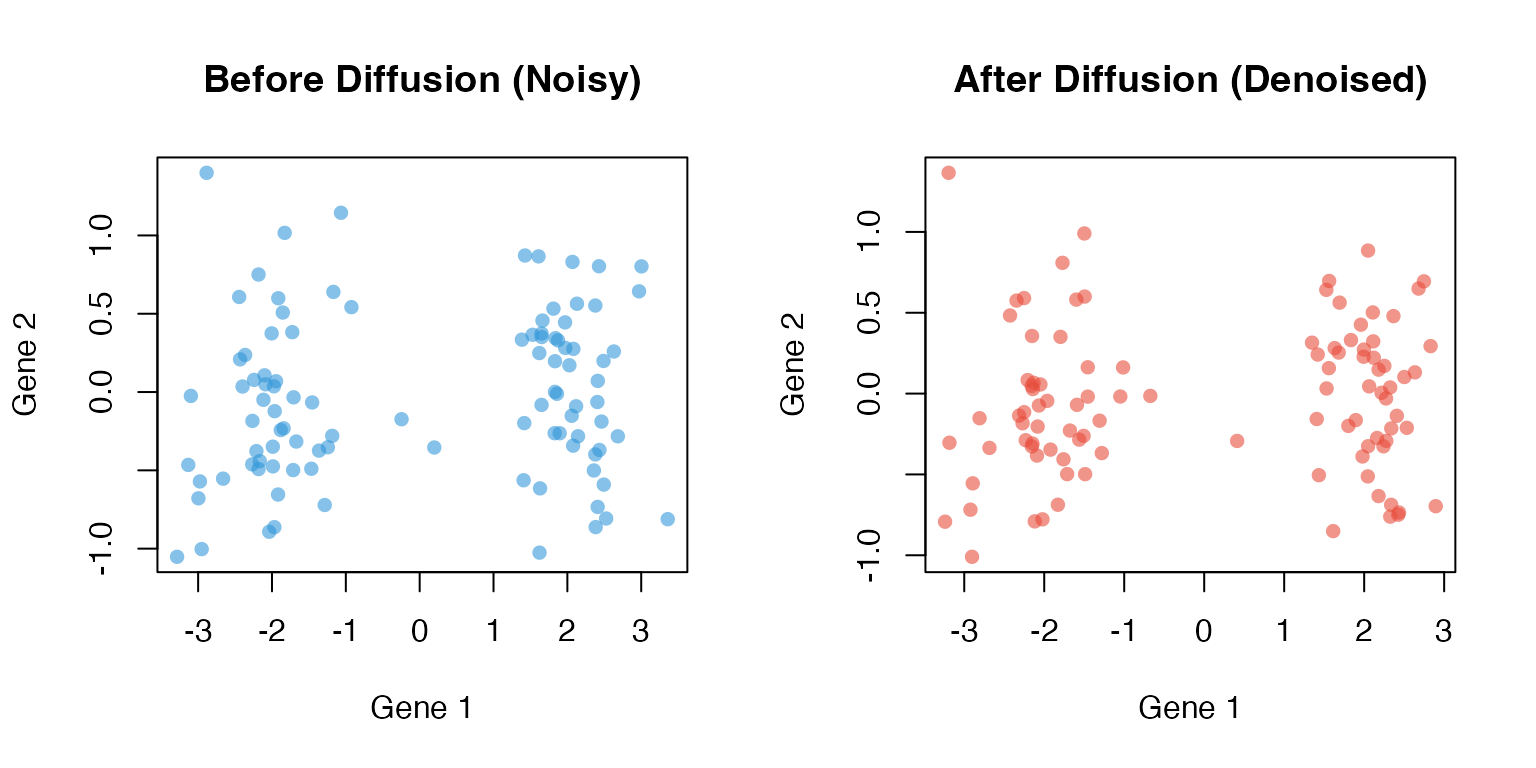

Automatic t Selection

When t = "auto", MAGIC uses Procrustes analysis to find optimal diffusion time.

Procrustes Disparity

Given two matrices $X$ and $Y$ , Procrustes analysis finds the optimal rotation $R$ that minimizes:

$d_{Procrustes}(X, Y) = \|X - YR\|_F^2$

after centering and normalizing both matrices.

Convergence Criterion

MAGIC iteratively applies diffusion and monitors:

$\Delta_t = d_{Procrustes}(X_t, X_{t+1})$

The algorithm stops when $\Delta_t < \theta$ (default: 0.001), indicating convergence.

library(MAGICR)
data(magic_testdata)

# Run with automatic t selection
result <- magic(magic_testdata, t = "auto", t_max = 15, verbose = TRUE)

cat("\nOptimal t selected:", result$params$t, "\n")
#> 
#> Optimal t selected: 15

Solver Options

Exact Solver

Computes imputation in full gene space:

$X_{imputed} = P^t X$

Advantages: - Preserves all gene-gene relationships - No approximation error

Disadvantages: - Memory intensive for large gene sets - Slower computation

Approximate Solver

Operates in PCA space and projects back:

$X_{imputed} = P^t X_{pca} \cdot V_k^T$

Advantages: - Much faster for large datasets - Lower memory footprint

Disadvantages: - Some information loss from PCA projection

Spectral Interpretation

The diffusion process has an elegant spectral interpretation. If $P$ has eigendecomposition:

$P = \sum_i \lambda_i v_i v_i^T$

Then:

$P^t = \sum_i \lambda_i^t v_i v_i^T$

Since $|\lambda_i| \leq 1$ :

Small eigenvalues (high-frequency noise) decay rapidly
Large eigenvalues (low-frequency signal) persist
Diffusion acts as a low-pass filter

Practical Recommendations

Parameter Selection Guidelines

Scenario	Recommended Parameters
Standard scRNA-seq	`t = 3-5`, `knn = 5`, `decay = 1`
Highly sparse data	`t = 5-10`, `knn = 10`
Rare populations	`t = 2-3`, `decay = 2`
Large datasets	`solver = "approximate"`, `npca = 50`

When to Use MAGIC

✅ Good use cases: - Visualizing gene-gene relationships - Trajectory analysis preprocessing - Recovering dropout in sparse data

❌ Avoid when: - Performing differential expression (use raw counts) - Data is already dense - Preserving exact count values is critical

References

van Dijk, D., et al. (2018). Recovering Gene Interactions from Single-Cell Data Using Data Diffusion. Cell, 174(3), 716-729.e27.
Coifman, R.R., & Lafon, S. (2006). Diffusion maps. Applied and Computational Harmonic Analysis, 21(1), 5-30.
Moon, K.R., et al. (2019). Visualizing structure and transitions in high-dimensional biological data. Nature Biotechnology, 37(12), 1482-1492.

Session Info

sessionInfo()
#> R version 4.4.0 (2024-04-24)
#> Platform: aarch64-apple-darwin20
#> Running under: macOS 15.6.1
#> 
#> Matrix products: default
#> BLAS:   /Library/Frameworks/R.framework/Versions/4.4-arm64/Resources/lib/libRblas.0.dylib 
#> LAPACK: /Library/Frameworks/R.framework/Versions/4.4-arm64/Resources/lib/libRlapack.dylib;  LAPACK version 3.12.0
#> 
#> locale:
#> [1] C
#> 
#> time zone: Asia/Shanghai
#> tzcode source: internal
#> 
#> attached base packages:
#> [1] stats     graphics  grDevices utils     datasets  methods   base     
#> 
#> other attached packages:
#> [1] MAGICR_1.0.0
#> 
#> loaded via a namespace (and not attached):
#>  [1] cli_3.6.5         knitr_1.51        rlang_1.1.7       xfun_0.56        
#>  [5] otel_0.2.0        textshaping_1.0.4 jsonlite_2.0.0    listenv_0.10.0   
#>  [9] htmltools_0.5.9   ragg_1.5.0        sass_0.4.10       rmarkdown_2.30   
#> [13] grid_4.4.0        evaluate_1.0.5    jquerylib_0.1.4   fastmap_1.2.0    
#> [17] yaml_2.3.12       lifecycle_1.0.5   compiler_4.4.0    codetools_0.2-20 
#> [21] irlba_2.3.5.1     fs_1.6.6          Rcpp_1.1.1        htmlwidgets_1.6.4
#> [25] future_1.69.0     lattice_0.22-7    systemfonts_1.3.1 digest_0.6.39    
#> [29] R6_2.6.1          RANN_2.6.2        parallelly_1.46.1 parallel_4.4.0   
#> [33] bslib_0.9.0       Matrix_1.7-4      tools_4.4.0       globals_0.18.0   
#> [37] pkgdown_2.1.3     cachem_1.1.0      desc_1.4.3

Zaoqu Liu

2026-01-26