Performance Benchmarking

Overview

This vignette benchmarks MAGICR performance across different data sizes and parameter configurations, helping users optimize their analysis workflow.

Setup

library(MAGICR)
library(Matrix)

# Helper function for timing
benchmark <- function(expr, name = "Operation") {
  start <- Sys.time()
  result <- eval(expr)
  elapsed <- as.numeric(difftime(Sys.time(), start, units = "secs"))
  cat(sprintf("%s: %.2f seconds\n", name, elapsed))
  invisible(list(result = result, time = elapsed))
}

Data Size Impact

Generating Test Data

# Generate sparse test matrices of varying sizes
generate_test_data <- function(n_cells, n_genes, sparsity = 0.9) {
  set.seed(42)
  data <- matrix(rpois(n_cells * n_genes, lambda = 2), 
                 nrow = n_cells, ncol = n_genes)
  data[runif(length(data)) < sparsity] <- 0
  colnames(data) <- paste0("Gene", seq_len(n_genes))
  rownames(data) <- paste0("Cell", seq_len(n_cells))
  data
}

# Test datasets
sizes <- list(
  small = c(100, 500),
  medium = c(500, 1000),
  large = c(1000, 2000)
)

Benchmarking Different Sizes

results <- list()

for (size_name in names(sizes)) {
  n_cells <- sizes[[size_name]][1]
  n_genes <- sizes[[size_name]][2]
  
  cat(sprintf("\n=== %s dataset: %d cells x %d genes ===\n", 
              size_name, n_cells, n_genes))
  
  test_data <- generate_test_data(n_cells, n_genes)
  
  # Benchmark
  bench <- benchmark(
    magic(test_data, t = 3, verbose = FALSE),
    name = sprintf("MAGIC (%s)", size_name)
  )
  
  results[[size_name]] <- bench$time
}
#> 
#> === small dataset: 100 cells x 500 genes ===
#> MAGIC (small): 0.04 seconds
#> 
#> === medium dataset: 500 cells x 1000 genes ===
#> MAGIC (medium): 1.29 seconds
#> 
#> === large dataset: 1000 cells x 2000 genes ===
#> MAGIC (large): 5.52 seconds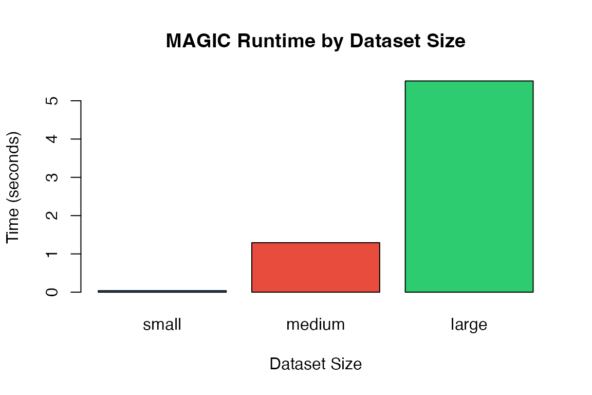

Visualization

# Plot timing results
barplot(unlist(results), 
        names.arg = names(results),
        col = c("#3498db", "#e74c3c", "#2ecc71"),
        main = "MAGIC Runtime by Dataset Size",
        ylab = "Time (seconds)",
        xlab = "Dataset Size")

Solver Comparison

Exact vs Approximate

# Medium-sized test data
test_data <- generate_test_data(500, 1000)

cat("=== Solver Comparison ===\n\n")
#> === Solver Comparison ===

# Exact solver
exact_bench <- benchmark(
  magic(test_data, t = 3, solver = "exact", verbose = FALSE),
  name = "Exact solver"
)
#> Exact solver: 1.34 seconds

# Approximate solver
approx_bench <- benchmark(
  magic(test_data, t = 3, solver = "approximate", npca = 50, verbose = FALSE),
  name = "Approximate solver"
)
#> Approximate solver: 0.50 seconds

cat(sprintf("\nSpeedup: %.1fx\n", exact_bench$time / approx_bench$time))
#> 
#> Speedup: 2.7x

Accuracy Comparison

# Compare results
exact_result <- as.matrix(exact_bench$result)
approx_result <- as.matrix(approx_bench$result)

# Correlation between methods
cor_val <- cor(as.vector(exact_result), as.vector(approx_result))
cat(sprintf("Correlation between exact and approximate: %.4f\n", cor_val))
#> Correlation between exact and approximate: 0.5631

# Visualization
par(mfrow = c(1, 2))

# Scatter plot
plot(as.vector(exact_result)[1:5000], 
     as.vector(approx_result)[1:5000],
     pch = 16, col = adjustcolor("#3498db", 0.3),
     xlab = "Exact Solver", ylab = "Approximate Solver",
     main = sprintf("Solver Agreement (r = %.3f)", cor_val))
abline(0, 1, col = "red", lwd = 2)

# Difference distribution
diff <- exact_result - approx_result
hist(as.vector(diff), breaks = 50, 
     main = "Difference Distribution",
     xlab = "Exact - Approximate",
     col = "#e74c3c", border = "white")
abline(v = 0, col = "black", lwd = 2, lty = 2)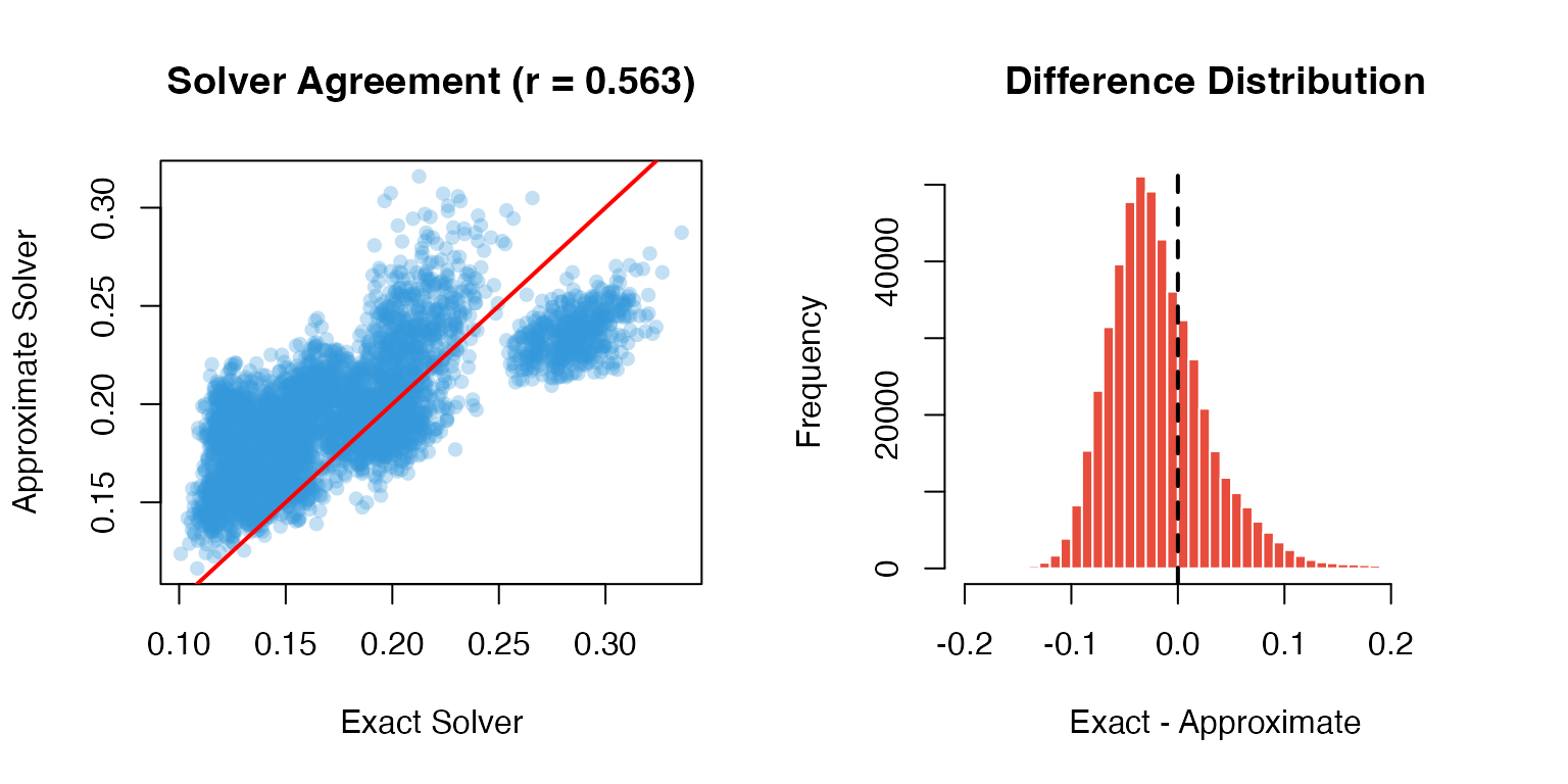

Parameter Impact

Effect of t (Diffusion Time)

test_data <- generate_test_data(200, 500)

t_values <- c(1, 2, 3, 5, 10)
t_times <- numeric(length(t_values))

for (i in seq_along(t_values)) {
  start <- Sys.time()
  magic(test_data, t = t_values[i], verbose = FALSE)
  t_times[i] <- as.numeric(difftime(Sys.time(), start, units = "secs"))
}

par(mfrow = c(1, 2))

# Runtime
plot(t_values, t_times, type = "b", pch = 16, col = "#3498db",
     xlab = "Diffusion Time (t)", ylab = "Runtime (seconds)",
     main = "Runtime vs Diffusion Time")

# Relative increase
plot(t_values, t_times / t_times[1], type = "b", pch = 16, col = "#e74c3c",
     xlab = "Diffusion Time (t)", ylab = "Relative Runtime",
     main = "Relative Runtime Increase")

Effect of knn

knn_values <- c(3, 5, 10, 15, 20)
knn_times <- numeric(length(knn_values))

for (i in seq_along(knn_values)) {
  start <- Sys.time()
  magic(test_data, t = 3, knn = knn_values[i], verbose = FALSE)
  knn_times[i] <- as.numeric(difftime(Sys.time(), start, units = "secs"))
}

plot(knn_values, knn_times, type = "b", pch = 16, col = "#2ecc71",
     xlab = "k-Nearest Neighbors", ylab = "Runtime (seconds)",
     main = "Runtime vs knn Parameter")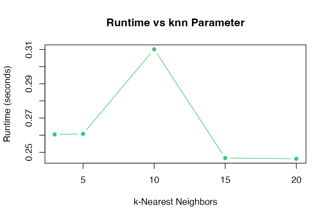

Effect of npca

npca_values <- c(20, 50, 100, 150)
npca_times <- numeric(length(npca_values))

for (i in seq_along(npca_values)) {
  start <- Sys.time()
  magic(test_data, t = 3, npca = npca_values[i], verbose = FALSE)
  npca_times[i] <- as.numeric(difftime(Sys.time(), start, units = "secs"))
}

plot(npca_values, npca_times, type = "b", pch = 16, col = "#9b59b6",
     xlab = "Number of PCA Components", ylab = "Runtime (seconds)",
     main = "Runtime vs npca Parameter")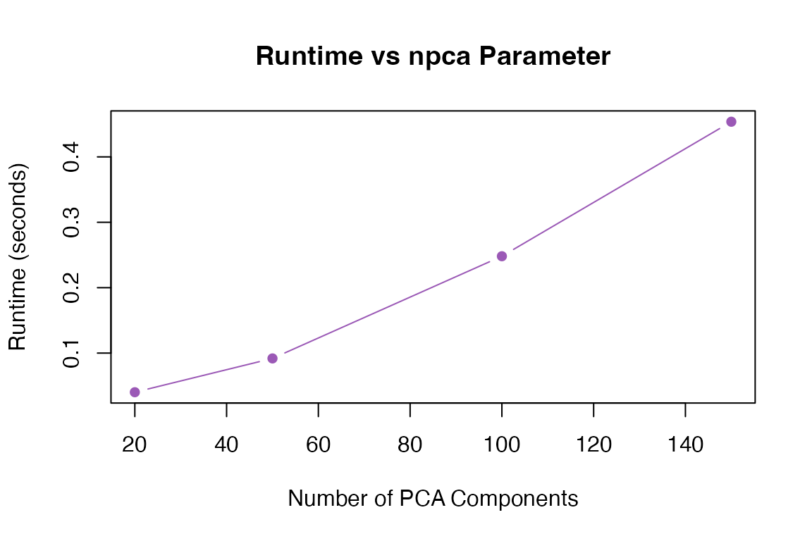

Memory Usage

Sparse vs Dense Input

# Create sparse and dense versions
test_dense <- generate_test_data(300, 800)
test_sparse <- Matrix::Matrix(test_dense, sparse = TRUE)

cat("=== Memory Comparison ===\n")
#> === Memory Comparison ===
cat(sprintf("Dense matrix size: %.2f MB\n", 
            object.size(test_dense) / 1024^2))
#> Dense matrix size: 1.90 MB
cat(sprintf("Sparse matrix size: %.2f MB\n", 
            object.size(test_sparse) / 1024^2))
#> Sparse matrix size: 0.31 MB
cat(sprintf("Compression ratio: %.1fx\n\n",
            as.numeric(object.size(test_dense)) / 
            as.numeric(object.size(test_sparse))))
#> Compression ratio: 6.1x

# Benchmark both
dense_bench <- benchmark(
  magic(test_dense, t = 3, verbose = FALSE),
  name = "Dense input"
)
#> Dense input: 0.61 seconds

sparse_bench <- benchmark(
  magic(test_sparse, t = 3, verbose = FALSE),
  name = "Sparse input"
)
#> Sparse input: 0.59 seconds

Recommendations

Based on benchmarking results:

Small Datasets (<1,000 cells)

# Use exact solver with default parameters
result <- magic(data, t = 3, solver = "exact")

Medium Datasets (1,000-10,000 cells)

# Consider approximate solver
result <- magic(data, t = 3, solver = "approximate", npca = 100)

Large Datasets (>10,000 cells)

# Use approximate solver with reduced PCA
# Enable parallel processing
library(future)
plan(multisession, workers = 4)

result <- magic(data, 
                t = 3, 
                solver = "approximate", 
                npca = 50,
                knn = 5)

Memory-Constrained Environments

# Use sparse matrices
# Reduce npca
# Impute only genes of interest
result <- magic(data,
                genes = important_genes,
                solver = "approximate",
                npca = 30)

Summary Table

Dataset Size	Recommended Solver	npca	Expected Time
<500 cells	exact	100	<5 sec
500-2000 cells	exact/approximate	100	5-30 sec
2000-10000 cells	approximate	50-100	30 sec - 5 min
>10000 cells	approximate + parallel	30-50	5-30 min

Session Info

sessionInfo()
#> R version 4.4.0 (2024-04-24)
#> Platform: aarch64-apple-darwin20
#> Running under: macOS 15.6.1
#> 
#> Matrix products: default
#> BLAS:   /Library/Frameworks/R.framework/Versions/4.4-arm64/Resources/lib/libRblas.0.dylib 
#> LAPACK: /Library/Frameworks/R.framework/Versions/4.4-arm64/Resources/lib/libRlapack.dylib;  LAPACK version 3.12.0
#> 
#> locale:
#> [1] C
#> 
#> time zone: Asia/Shanghai
#> tzcode source: internal
#> 
#> attached base packages:
#> [1] stats     graphics  grDevices utils     datasets  methods   base     
#> 
#> other attached packages:
#> [1] Matrix_1.7-4 MAGICR_1.0.0
#> 
#> loaded via a namespace (and not attached):
#>  [1] cli_3.6.5         knitr_1.51        rlang_1.1.7       xfun_0.56        
#>  [5] otel_0.2.0        textshaping_1.0.4 jsonlite_2.0.0    listenv_0.10.0   
#>  [9] htmltools_0.5.9   ragg_1.5.0        sass_0.4.10       rmarkdown_2.30   
#> [13] grid_4.4.0        evaluate_1.0.5    jquerylib_0.1.4   fastmap_1.2.0    
#> [17] yaml_2.3.12       lifecycle_1.0.5   compiler_4.4.0    codetools_0.2-20 
#> [21] irlba_2.3.5.1     fs_1.6.6          Rcpp_1.1.1        htmlwidgets_1.6.4
#> [25] future_1.69.0     lattice_0.22-7    systemfonts_1.3.1 digest_0.6.39    
#> [29] R6_2.6.1          RANN_2.6.2        parallelly_1.46.1 parallel_4.4.0   
#> [33] bslib_0.9.0       tools_4.4.0       globals_0.18.0    pkgdown_2.1.3    
#> [37] cachem_1.1.0      desc_1.4.3

Zaoqu Liu

2026-01-26

Overview

Setup

Data Size Impact

Generating Test Data

Benchmarking Different Sizes

Visualization

Solver Comparison

Exact vs Approximate

Accuracy Comparison

Parameter Impact

Effect of t (Diffusion Time)

Effect of knn

Effect of npca

Memory Usage

Sparse vs Dense Input

Recommendations

Small Datasets (<1,000 cells)

Medium Datasets (1,000-10,000 cells)

Large Datasets (>10,000 cells)

Memory-Constrained Environments

Summary Table

Session Info