Bulk RNA-seq Metabolic Flux Analysis
Zaoqu Liu
2026-01-23
Source:vignettes/bulk_analysis.Rmd
bulk_analysis.RmdOverview
This vignette demonstrates the complete workflow for metabolic flux analysis from bulk RNA-seq data using METAFLUX.
Load Package and Data
library(METAFLUX)
library(ggplot2)

# Load example bulk RNA-seq data
data("bulk_test_example")
data("human_blood")
data("human_gem")

# Inspect data
cat("Gene expression matrix:\n")
#> Gene expression matrix:
cat("  Dimensions:", dim(bulk_test_example), "\n")
#>   Dimensions: 58581 5
cat("  Samples:", colnames(bulk_test_example), "\n")
#>   Samples: Sample1 Sample2 Sample3 Sample4 Sample5
cat("  Example genes:", head(rownames(bulk_test_example), 5), "\n")
#>   Example genes: TSPAN6 TNMD DPM1 SCYL3 C1orf112
Step 1: Calculate MRAS
Metabolic Reaction Activity Scores (MRAS) integrate gene expression with metabolic network topology.
# Calculate MRAS
mras <- calculate_reaction_score(bulk_test_example)

# Check output
cat("\nMRAS matrix:\n")
#>
#> MRAS matrix:
cat("  Dimensions:", dim(mras), "\n")
#>   Dimensions: 13082 5
cat("  Score range:", range(as.matrix(mras)), "\n")
#>   Score range: 0 1
MRAS Distribution
mras_values <- as.vector(as.matrix(mras))
mras_df <- data.frame(MRAS = mras_values[mras_values > 0])

ggplot(mras_df, aes(x = MRAS)) +
  geom_histogram(bins = 50, fill = "#3498db", color = "white", alpha = 0.8) +
  labs(
    title = "Distribution of Metabolic Reaction Activity Scores",
    x = "MRAS Value",
    y = "Count"
  ) +
  theme_minimal() +
  theme(plot.title = element_text(hjust = 0.5, face = "bold"))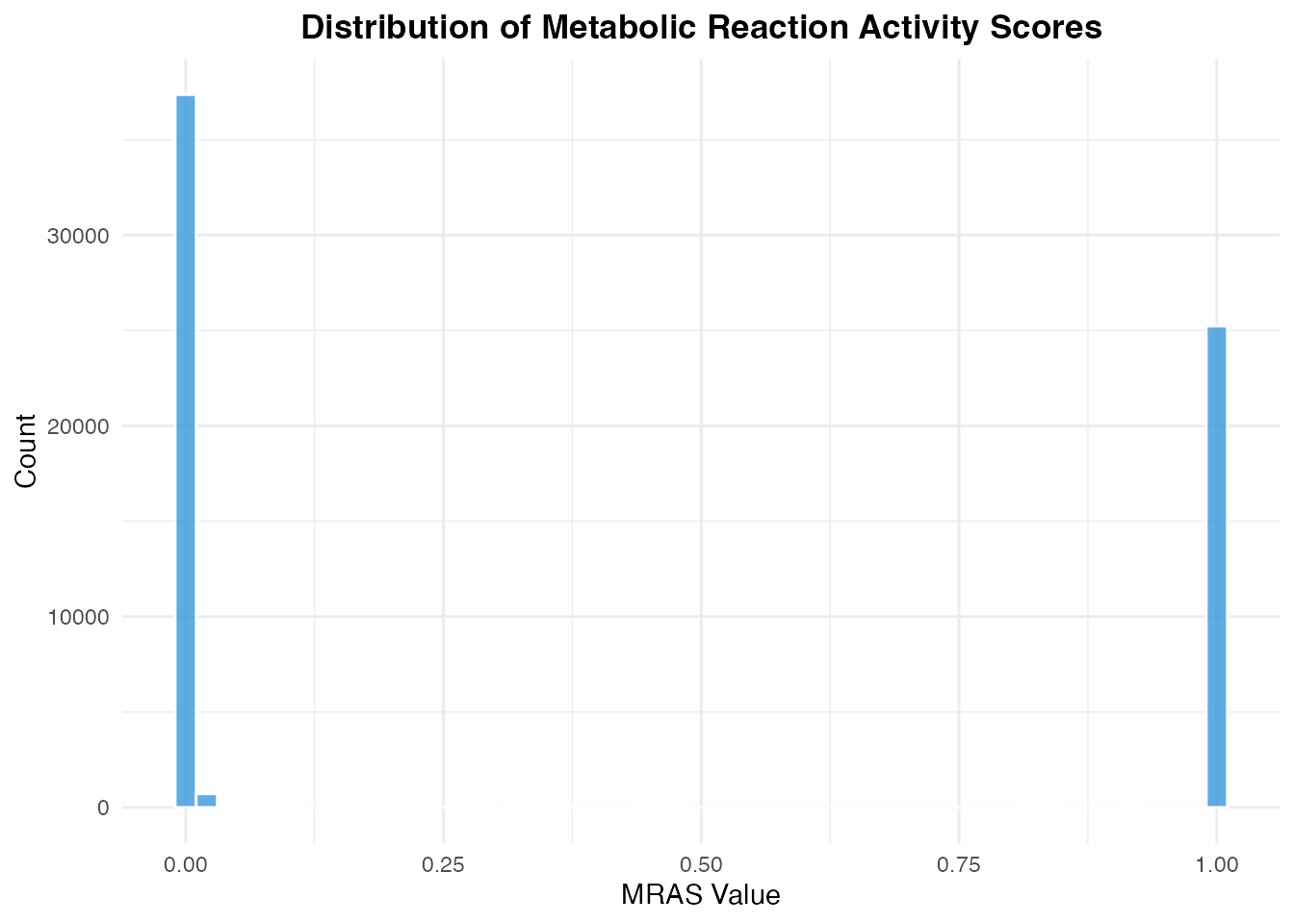
Distribution of MRAS values
Step 2: Compute Metabolic Fluxes
# Run flux balance analysis
flux <- compute_flux(mras = mras, medium = human_blood)
#>   |                                                                              |                                                                      |   0%  |                                                                              |==============                                                        |  20%  |                                                                              |============================                                          |  40%  |                                                                              |==========================================                            |  60%  |                                                                              |========================================================              |  80%  |                                                                              |======================================================================| 100%

# Check results
cat("\nFlux matrix:\n")
#>
#> Flux matrix:
cat("  Dimensions:", dim(flux), "\n")
#>   Dimensions: 13082 5
cat("  Flux range:", range(flux), "\n")
#>   Flux range: -0.08404168 0.08406293
Flux Interpretation
# Classify reactions by flux direction
flux_mean <- rowMeans(flux)
flux_class <- data.frame(
  Direction = c("Production (+)", "Consumption (-)", "Inactive (≈0)"),
  Count = c(
    sum(flux_mean > 0.001),
    sum(flux_mean < -0.001),
    sum(abs(flux_mean) <= 0.001)
  )
)

ggplot(flux_class, aes(x = Direction, y = Count, fill = Direction)) +
  geom_bar(stat = "identity", width = 0.6) +
  geom_text(aes(label = Count), vjust = -0.5, size = 5) +
  scale_fill_manual(values = c("#27ae60", "#e74c3c", "#95a5a6")) +
  labs(
    title = "Reaction Classification by Flux Direction",
    x = "",
    y = "Number of Reactions"
  ) +
  theme_minimal() +
  theme(
    plot.title = element_text(hjust = 0.5, face = "bold"),
    legend.position = "none"
  ) +
  ylim(0, max(flux_class$Count) * 1.1)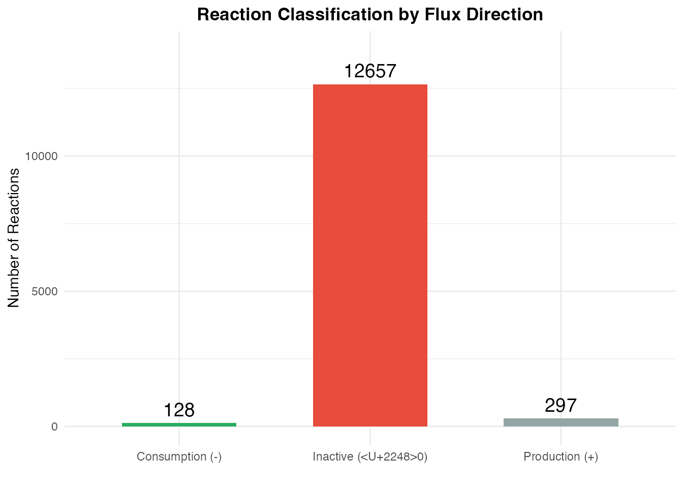
Interpretation of flux values
Step 3: Key Metabolic Indicators
Central Carbon Metabolism
# Define key reactions
central_carbon <- c(
  "Glucose uptake" = "HMR_9034",
  "Lactate secretion" = "HMR_9135",
  "Pyruvate transport" = "HMR_9133",
  "Glutamine uptake" = "HMR_9063"
)

# Extract and plot
cc_flux <- flux[central_carbon, , drop = FALSE]
rownames(cc_flux) <- names(central_carbon)

cc_df <- data.frame(
  Reaction = rep(rownames(cc_flux), ncol(cc_flux)),
  Sample = rep(colnames(cc_flux), each = nrow(cc_flux)),
  Flux = as.vector(as.matrix(cc_flux))
)

ggplot(cc_df, aes(x = Reaction, y = Flux, fill = Sample)) +
  geom_bar(stat = "identity", position = "dodge") +
  geom_hline(yintercept = 0, linetype = "dashed") +
  scale_fill_brewer(palette = "Set2") +
  labs(
    title = "Central Carbon Metabolism",
    subtitle = "Key reaction fluxes across samples",
    x = "",
    y = "Flux"
  ) +
  theme_minimal() +
  theme(
    plot.title = element_text(hjust = 0.5, face = "bold"),
    axis.text.x = element_text(angle = 30, hjust = 1)
  )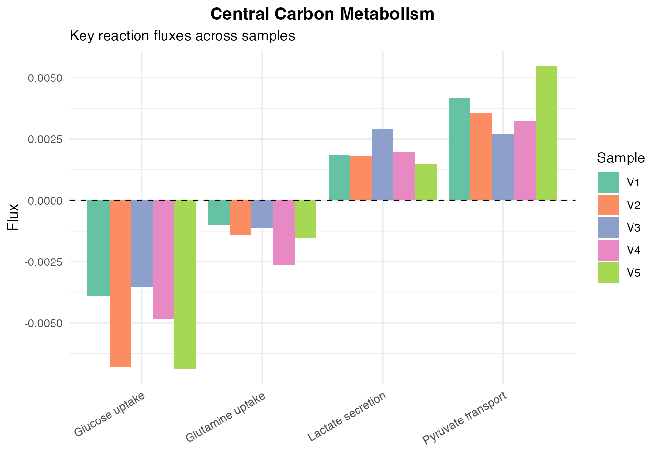
Central carbon metabolism flux
Biomass Production
biomass_flux <- flux["biomass_human", ]

biomass_df <- data.frame(
  Sample = names(biomass_flux),
  Flux = as.numeric(biomass_flux)
)

ggplot(biomass_df, aes(x = Sample, y = Flux, fill = Sample)) +
  geom_bar(stat = "identity", width = 0.6) +
  scale_fill_brewer(palette = "Set2") +
  labs(
    title = "Biomass Production Rate",
    subtitle = "Proxy for cellular growth rate",
    x = "Sample",
    y = "Biomass Flux"
  ) +
  theme_minimal() +
  theme(
    plot.title = element_text(hjust = 0.5, face = "bold"),
    legend.position = "none"
  )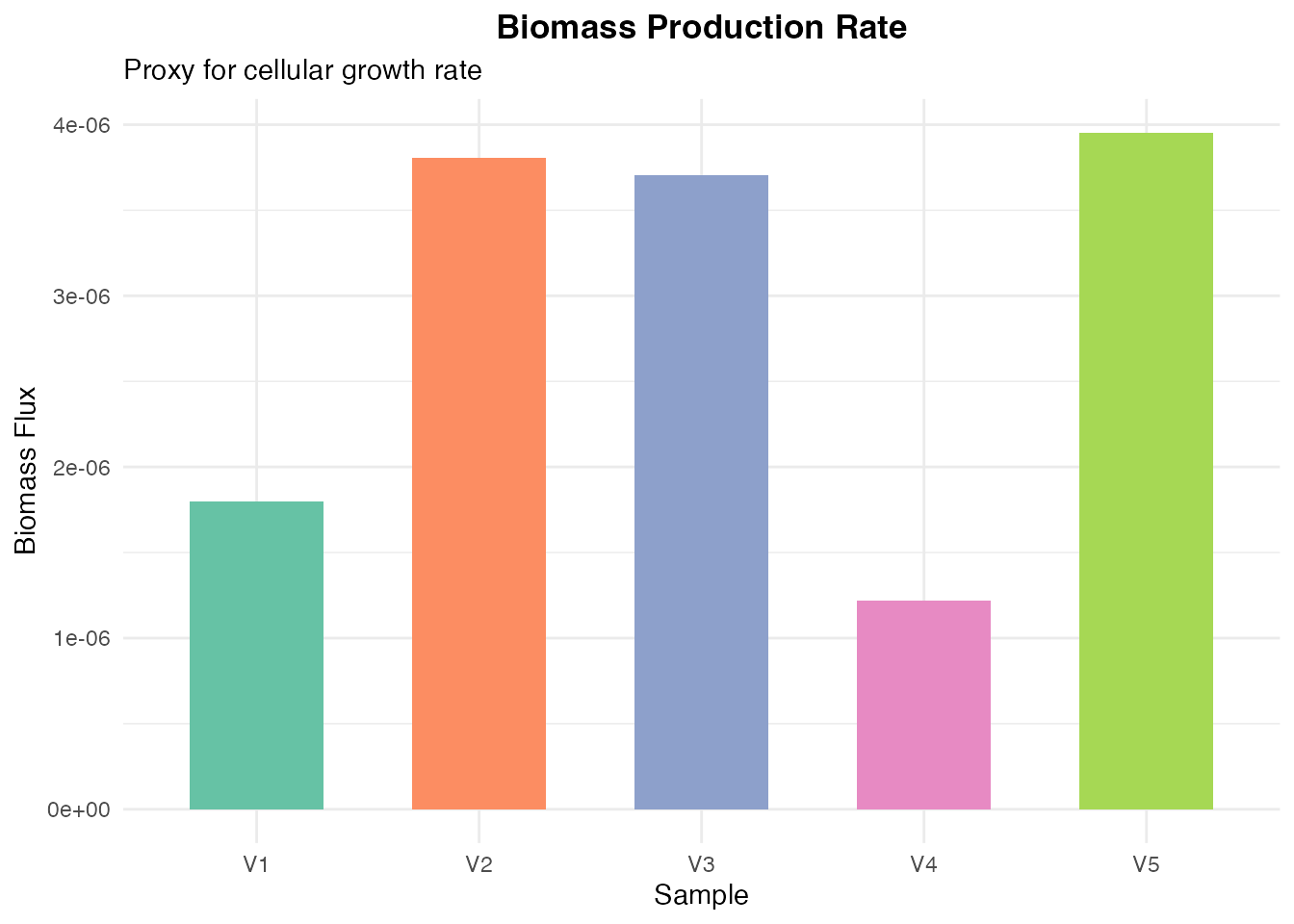
Biomass production flux (growth rate proxy)
Step 4: Pathway Analysis
# Map reactions to pathways
pathway_map <- human_gem$SUBSYSTEM
names(pathway_map) <- human_gem$ID

# Calculate pathway activity
pathways <- unique(pathway_map)
pathway_activity <- sapply(pathways, function(pw) {
  rxns <- names(pathway_map)[pathway_map == pw]
  rxns <- intersect(rxns, rownames(flux))
  if (length(rxns) > 0) mean(abs(flux[rxns, ])) else NA
})

# Top 12 pathways
top_pw <- sort(pathway_activity[!is.na(pathway_activity)], decreasing = TRUE)[1:12]

pw_df <- data.frame(
  Pathway = factor(names(top_pw), levels = rev(names(top_pw))),
  Activity = top_pw
)

ggplot(pw_df, aes(x = Activity, y = Pathway)) +
  geom_bar(stat = "identity", fill = "#2c3e50") +
  labs(
    title = "Top 12 Active Metabolic Pathways",
    x = "Mean Absolute Flux",
    y = ""
  ) +
  theme_minimal() +
  theme(
    plot.title = element_text(hjust = 0.5, face = "bold"),
    axis.text.y = element_text(size = 9)
  )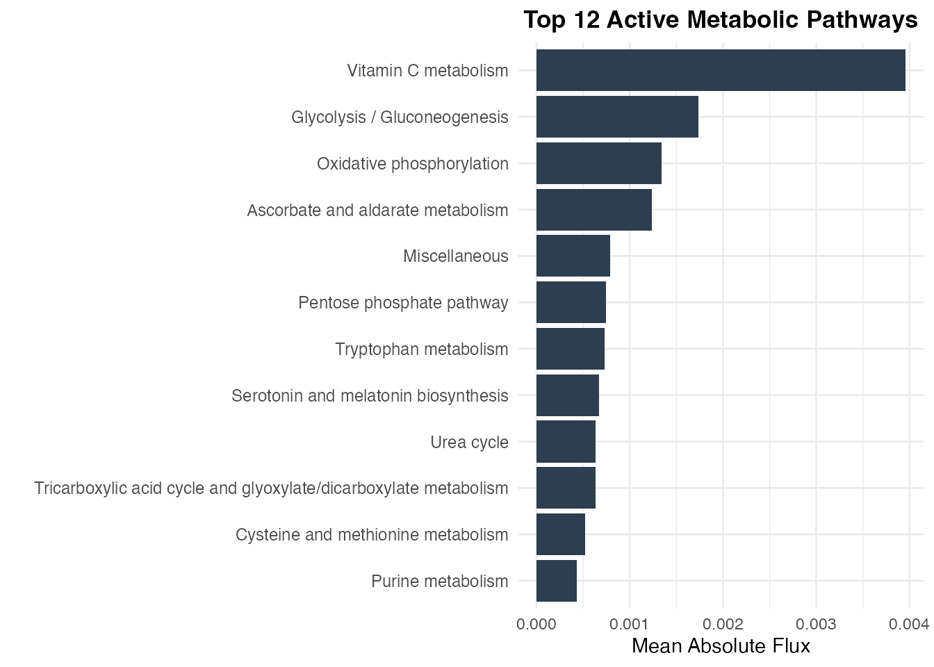
Top metabolic pathways by activity
Step 5: Quality Control
Steady-State Verification
# Load stoichiometric matrix
Hgem <- METAFLUX:::Hgem

# Check steady-state constraint: S*v = 0
sv_violations <- sapply(1:ncol(flux), function(i) {
  sv <- Hgem$S %*% flux[, i]
  max(abs(sv))
})

cat("Steady-state constraint check:\n")
#> Steady-state constraint check:
cat("  Max violations per sample:", round(sv_violations, 6), "\n")
#>   Max violations per sample: 2.3e-05 7e-06 1.4e-05 1.7e-05 1.3e-05
cat("  All < 0.001:", all(sv_violations < 0.001), "\n")
#>   All < 0.001: TRUE
Gene Coverage
gene_num <- METAFLUX:::gene_num
input_genes <- rownames(bulk_test_example)
metabolic_genes <- rownames(gene_num)

coverage <- sum(input_genes %in% metabolic_genes)
total <- length(metabolic_genes)

cov_df <- data.frame(
  Category = c("Detected", "Missing"),
  Count = c(coverage, total - coverage)
)

ggplot(cov_df, aes(x = "", y = Count, fill = Category)) +
  geom_bar(stat = "identity", width = 1) +
  coord_polar("y") +
  scale_fill_manual(values = c("Detected" = "#27ae60", "Missing" = "#e74c3c")) +
  labs(
    title = "Metabolic Gene Coverage",
    subtitle = sprintf("%.1f%% (%d/%d genes)", coverage/total*100, coverage, total)
  ) +
  theme_void() +
  theme(
    plot.title = element_text(hjust = 0.5, face = "bold"),
    plot.subtitle = element_text(hjust = 0.5)
  )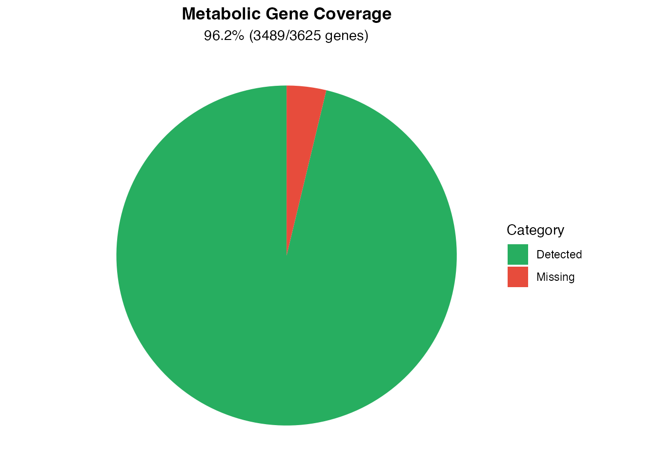
Metabolic gene coverage
Summary
cat("================================================\n")
#> ================================================
cat("METAFLUX Bulk RNA-seq Analysis Complete\n")
#> METAFLUX Bulk RNA-seq Analysis Complete
cat("================================================\n\n")
#> ================================================

cat("Input:\n")
#> Input:
cat(sprintf("  Genes: %d\n", nrow(bulk_test_example)))
#>   Genes: 58581
cat(sprintf("  Samples: %d\n", ncol(bulk_test_example)))
#>   Samples: 5
cat(sprintf("  Metabolic gene coverage: %.1f%%\n", coverage/total*100))
#>   Metabolic gene coverage: 96.2%

cat("\nOutput:\n")
#>
#> Output:
cat(sprintf("  Reactions: %d\n", nrow(flux)))
#>   Reactions: 13082
cat(sprintf("  Flux range: [%.4f, %.4f]\n", min(flux), max(flux)))
#>   Flux range: [-0.0840, 0.0841]

cat("\nKey findings:\n")
#>
#> Key findings:
cat(sprintf("  Active reactions: %d\n", sum(abs(rowMeans(flux)) > 0.001)))
#>   Active reactions: 425
cat(sprintf("  Glucose uptake (mean): %.4f\n", mean(flux["HMR_9034", ])))
#>   Glucose uptake (mean): -0.0052
cat(sprintf("  Lactate secretion (mean): %.4f\n", mean(flux["HMR_9135", ])))
#>   Lactate secretion (mean): 0.0020
Author
Zaoqu Liu - Package maintainer and developer
- GitHub: Zaoqu-Liu
- ORCID: 0000-0002-0452-742X
- Email: liuzaoqu@163.com
Session Information
sessionInfo()
#> R version 4.4.0 (2024-04-24)
#> Platform: aarch64-apple-darwin20
#> Running under: macOS 15.6.1
#>
#> Matrix products: default
#> BLAS:   /Library/Frameworks/R.framework/Versions/4.4-arm64/Resources/lib/libRblas.0.dylib
#> LAPACK: /Library/Frameworks/R.framework/Versions/4.4-arm64/Resources/lib/libRlapack.dylib;  LAPACK version 3.12.0
#>
#> locale:
#> [1] C
#>
#> time zone: Asia/Shanghai
#> tzcode source: internal
#>
#> attached base packages:
#> [1] stats     graphics  grDevices utils     datasets  methods   base
#>
#> other attached packages:
#> [1] ggplot2_4.0.1  METAFLUX_2.2.0
#>
#> loaded via a namespace (and not attached):
#>   [1] deldir_2.0-4           pbapply_1.7-4          gridExtra_2.3
#>   [4] rlang_1.1.7            magrittr_2.0.4         RcppAnnoy_0.0.23
#>   [7] otel_0.2.0             spatstat.geom_3.6-1    matrixStats_1.5.0
#>  [10] ggridges_0.5.7         compiler_4.4.0         png_0.1-8
#>  [13] systemfonts_1.3.1      vctrs_0.7.0            reshape2_1.4.5
#>  [16] stringr_1.6.0          pkgconfig_2.0.3        fastmap_1.2.0
#>  [19] labeling_0.4.3         promises_1.5.0         rmarkdown_2.30
#>  [22] ragg_1.5.0             purrr_1.2.1            xfun_0.56
#>  [25] cachem_1.1.0           jsonlite_2.0.0         goftest_1.2-3
#>  [28] later_1.4.5            spatstat.utils_3.2-1   irlba_2.3.5.1
#>  [31] parallel_4.4.0         cluster_2.1.8.1        R6_2.6.1
#>  [34] ica_1.0-3              spatstat.data_3.1-9    bslib_0.9.0
#>  [37] stringi_1.8.7          RColorBrewer_1.1-3     reticulate_1.44.1
#>  [40] spatstat.univar_3.1-6  parallelly_1.46.1      lmtest_0.9-40
#>  [43] jquerylib_0.1.4        scattermore_1.2        iterators_1.0.14
#>  [46] Rcpp_1.1.1             knitr_1.51             tensor_1.5.1
#>  [49] future.apply_1.20.1    zoo_1.8-15             sctransform_0.4.3
#>  [52] httpuv_1.6.16          Matrix_1.7-4           splines_4.4.0
#>  [55] igraph_2.2.1           tidyselect_1.2.1       abind_1.4-8
#>  [58] dichromat_2.0-0.1      yaml_2.3.12            doParallel_1.0.17
#>  [61] spatstat.random_3.4-3  spatstat.explore_3.6-0 codetools_0.2-20
#>  [64] miniUI_0.1.2           listenv_0.10.0         plyr_1.8.9
#>  [67] lattice_0.22-7         tibble_3.3.1           withr_3.0.2
#>  [70] shiny_1.12.1           S7_0.2.1               ROCR_1.0-11
#>  [73] evaluate_1.0.5         Rtsne_0.17             future_1.69.0
#>  [76] desc_1.4.3             survival_3.8-3         polyclip_1.10-7
#>  [79] fitdistrplus_1.2-4     osqp_0.6.3.3           pillar_1.11.1
#>  [82] Seurat_4.4.0           KernSmooth_2.23-26     foreach_1.5.2
#>  [85] plotly_4.11.0          generics_0.1.4         sp_2.2-0
#>  [88] scales_1.4.0           globals_0.18.0         xtable_1.8-4
#>  [91] glue_1.8.0             lazyeval_0.2.2         tools_4.4.0
#>  [94] data.table_1.18.0      RANN_2.6.2             fs_1.6.6
#>  [97] leiden_0.4.3.1         cowplot_1.2.0          grid_4.4.0
#> [100] tidyr_1.3.2            nlme_3.1-168           patchwork_1.3.2
#> [103] cli_3.6.5              spatstat.sparse_3.1-0  textshaping_1.0.4
#> [106] viridisLite_0.4.2      dplyr_1.1.4            uwot_0.2.4
#> [109] gtable_0.3.6           sass_0.4.10            digest_0.6.39
#> [112] progressr_0.18.0       ggrepel_0.9.6          htmlwidgets_1.6.4
#> [115] SeuratObject_4.1.4     farver_2.1.2           htmltools_0.5.9
#> [118] pkgdown_2.1.3          lifecycle_1.0.5        httr_1.4.7
#> [121] mime_0.13              MASS_7.3-65