Visualization Guide for METAFLUX
Zaoqu Liu
2026-01-23
Source:vignettes/visualization.Rmd
visualization.RmdStep 1: Calculate MRAS
# Calculate Metabolic Reaction Activity Scores
mras <- calculate_reaction_score(bulk_test_example)
cat("MRAS matrix:", nrow(mras), "reactions x", ncol(mras), "samples\n")
#> MRAS matrix: 13082 reactions x 5 samples
Step 2: Compute Fluxes
# Compute metabolic fluxes
flux <- compute_flux(mras = mras, medium = human_blood)
#>   |                                                                              |                                                                      |   0%  |                                                                              |==============                                                        |  20%  |                                                                              |============================                                          |  40%  |                                                                              |==========================================                            |  60%  |                                                                              |========================================================              |  80%  |                                                                              |======================================================================| 100%
cat("Flux matrix:", nrow(flux), "reactions x", ncol(flux), "samples\n")
#> Flux matrix: 13082 reactions x 5 samples
Visualization 1: Flux Distribution
# Prepare data
flux_values <- as.vector(as.matrix(flux))
flux_df <- data.frame(flux = flux_values[abs(flux_values) < 0.5])

# Plot
ggplot(flux_df, aes(x = flux)) +
  geom_histogram(bins = 100, fill = "#3498db", color = "white", alpha = 0.8) +
  labs(
    title = "Distribution of Metabolic Fluxes",
    subtitle = "METAFLUX analysis of bulk RNA-seq data",
    x = "Flux Value",
    y = "Count"
  ) +
  theme_minimal() +
  theme(
    plot.title = element_text(hjust = 0.5, size = 14, face = "bold"),
    plot.subtitle = element_text(hjust = 0.5, size = 10, color = "gray50")
  )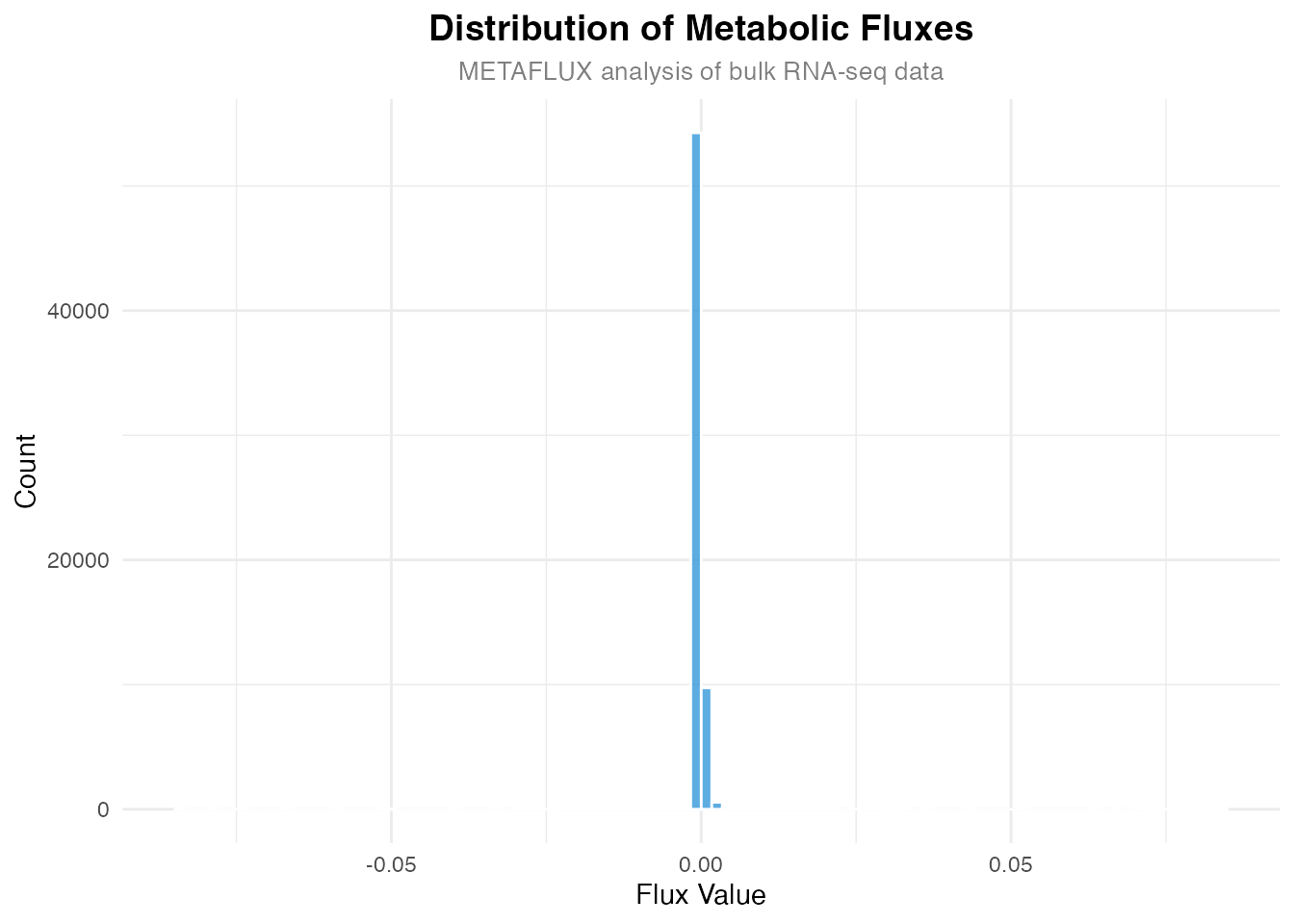
Distribution of metabolic fluxes across all samples
Visualization 2: Key Metabolite Exchange
# Define key reactions
key_rxns <- c(
  "Glucose" = "HMR_9034",
  "Lactate" = "HMR_9135",
  "Glutamine" = "HMR_9063",
  "Pyruvate" = "HMR_9133"
)

# Extract flux values
key_flux <- flux[key_rxns, , drop = FALSE]
rownames(key_flux) <- names(key_rxns)

# Convert to long format
key_df <- data.frame(
  Metabolite = rep(rownames(key_flux), ncol(key_flux)),
  Sample = rep(colnames(key_flux), each = nrow(key_flux)),
  Flux = as.vector(as.matrix(key_flux))
)

# Plot
ggplot(key_df, aes(x = Metabolite, y = Flux, fill = Sample)) +
  geom_bar(stat = "identity", position = "dodge", width = 0.7) +
  geom_hline(yintercept = 0, linetype = "dashed", color = "gray50") +
  labs(
    title = "Key Metabolite Exchange",
    subtitle = "Negative = uptake, Positive = secretion",
    x = "",
    y = "Flux"
  ) +
  scale_fill_brewer(palette = "Set2") +
  theme_minimal() +
  theme(
    plot.title = element_text(hjust = 0.5, size = 14, face = "bold"),
    plot.subtitle = element_text(hjust = 0.5, size = 10, color = "gray50"),
    axis.text.x = element_text(angle = 45, hjust = 1, size = 11)
  )
Flux values for key metabolic reactions
Visualization 3: Top Variable Reactions
# Calculate variance
flux_var <- apply(flux, 1, var)
top_30 <- names(sort(flux_var, decreasing = TRUE)[1:30])

# Prepare matrix
flux_top <- as.matrix(flux[top_30, ])

# Scale for visualization
flux_scaled <- t(scale(t(flux_top)))

# Convert to data frame
heatmap_df <- data.frame(
  Reaction = rep(rownames(flux_scaled), ncol(flux_scaled)),
  Sample = rep(colnames(flux_scaled), each = nrow(flux_scaled)),
  Flux = as.vector(flux_scaled)
)

# Order reactions by mean flux
rxn_order <- rownames(flux_scaled)[order(rowMeans(flux_scaled))]
heatmap_df$Reaction <- factor(heatmap_df$Reaction, levels = rxn_order)

# Plot heatmap
ggplot(heatmap_df, aes(x = Sample, y = Reaction, fill = Flux)) +
  geom_tile() +
  scale_fill_gradient2(
    low = "#2166ac", mid = "white", high = "#b2182b",
    midpoint = 0, name = "Z-score"
  ) +
  labs(
    title = "Top 30 Variable Metabolic Reactions",
    x = "Sample",
    y = "Reaction"
  ) +
  theme_minimal() +
  theme(
    plot.title = element_text(hjust = 0.5, size = 14, face = "bold"),
    axis.text.y = element_text(size = 6),
    axis.text.x = element_text(angle = 45, hjust = 1)
  )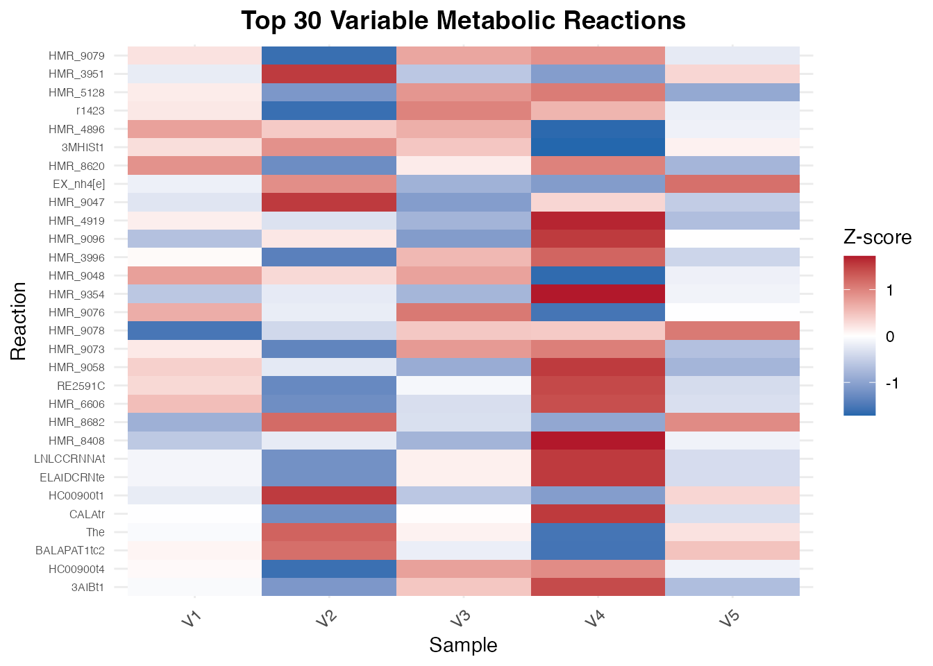
Heatmap of top 30 most variable metabolic reactions
Visualization 4: Pathway Activity
# Get pathway information
pathway_map <- human_gem$SUBSYSTEM
names(pathway_map) <- human_gem$ID

# Calculate mean flux per pathway
flux_matrix <- as.matrix(flux)
pathways <- unique(pathway_map)

pathway_flux <- sapply(pathways, function(pw) {
  rxns <- names(pathway_map)[pathway_map == pw]
  rxns <- intersect(rxns, rownames(flux_matrix))
  if (length(rxns) > 0) {
    mean(abs(flux_matrix[rxns, ]), na.rm = TRUE)
  } else {
    NA
  }
})

# Remove NA and get top 15
pathway_flux <- sort(pathway_flux[!is.na(pathway_flux)], decreasing = TRUE)
top_pathways <- head(pathway_flux, 15)

# Create data frame
pathway_df <- data.frame(
  Pathway = factor(names(top_pathways), levels = rev(names(top_pathways))),
  Activity = top_pathways
)

# Plot
ggplot(pathway_df, aes(x = Activity, y = Pathway)) +
  geom_bar(stat = "identity", fill = "#2c3e50", width = 0.7) +
  labs(
    title = "Top 15 Active Metabolic Pathways",
    subtitle = "Based on mean absolute flux",
    x = "Mean Absolute Flux",
    y = ""
  ) +
  theme_minimal() +
  theme(
    plot.title = element_text(hjust = 0.5, size = 14, face = "bold"),
    plot.subtitle = element_text(hjust = 0.5, size = 10, color = "gray50"),
    axis.text.y = element_text(size = 9)
  )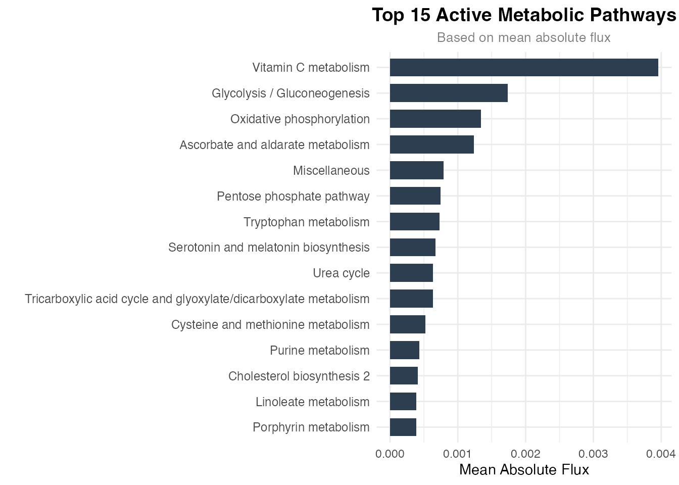
Mean absolute flux by metabolic pathway (top 15)
Visualization 5: Sample Correlation
# Calculate correlation
cor_matrix <- cor(as.matrix(flux), use = "pairwise.complete.obs")

# Convert to long format
cor_df <- data.frame(
  Sample1 = rep(rownames(cor_matrix), ncol(cor_matrix)),
  Sample2 = rep(colnames(cor_matrix), each = nrow(cor_matrix)),
  Correlation = as.vector(cor_matrix)
)

# Plot
ggplot(cor_df, aes(x = Sample1, y = Sample2, fill = Correlation)) +
  geom_tile() +
  geom_text(aes(label = round(Correlation, 2)), size = 4) +
  scale_fill_gradient2(
    low = "#2166ac", mid = "white", high = "#b2182b",
    midpoint = 0.5, limits = c(0, 1)
  ) +
  labs(
    title = "Sample Correlation Matrix",
    subtitle = "Based on metabolic flux profiles",
    x = "", y = ""
  ) +
  theme_minimal() +
  theme(
    plot.title = element_text(hjust = 0.5, size = 14, face = "bold"),
    plot.subtitle = element_text(hjust = 0.5, size = 10, color = "gray50"),
    axis.text.x = element_text(angle = 45, hjust = 1)
  )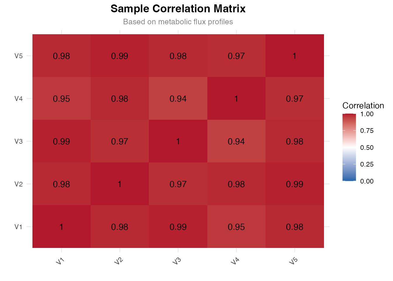
Correlation matrix of metabolic flux profiles
Visualization 6: Exchange Reaction Analysis
# Identify exchange reactions
exchange_idx <- grep("Exchange", human_gem$SUBSYSTEM)
exchange_rxns <- human_gem$ID[exchange_idx]
exchange_rxns <- intersect(exchange_rxns, rownames(flux))

# Get mean flux
exchange_flux <- rowMeans(flux[exchange_rxns, ])

# Classify
exchange_df <- data.frame(
  Reaction = names(exchange_flux),
  Flux = exchange_flux,
  Type = ifelse(exchange_flux < -0.001, "Uptake",
                ifelse(exchange_flux > 0.001, "Secretion", "Inactive"))
)

# Summary counts
type_counts <- table(exchange_df$Type)
cat("\nExchange reaction summary:\n")
#>
#> Exchange reaction summary:
print(type_counts)
#>
#>  Inactive Secretion    Uptake
#>      1598        27        23

# Plot distribution
ggplot(exchange_df[exchange_df$Type != "Inactive", ],
       aes(x = Flux, fill = Type)) +
  geom_histogram(bins = 50, alpha = 0.7, position = "identity") +
  scale_fill_manual(values = c("Uptake" = "#e74c3c", "Secretion" = "#27ae60")) +
  labs(
    title = "Exchange Reaction Distribution",
    subtitle = sprintf("Uptake: %d, Secretion: %d, Inactive: %d",
                      type_counts["Uptake"], type_counts["Secretion"],
                      type_counts["Inactive"]),
    x = "Mean Flux",
    y = "Count"
  ) +
  theme_minimal() +
  theme(
    plot.title = element_text(hjust = 0.5, size = 14, face = "bold"),
    plot.subtitle = element_text(hjust = 0.5, size = 10, color = "gray50")
  )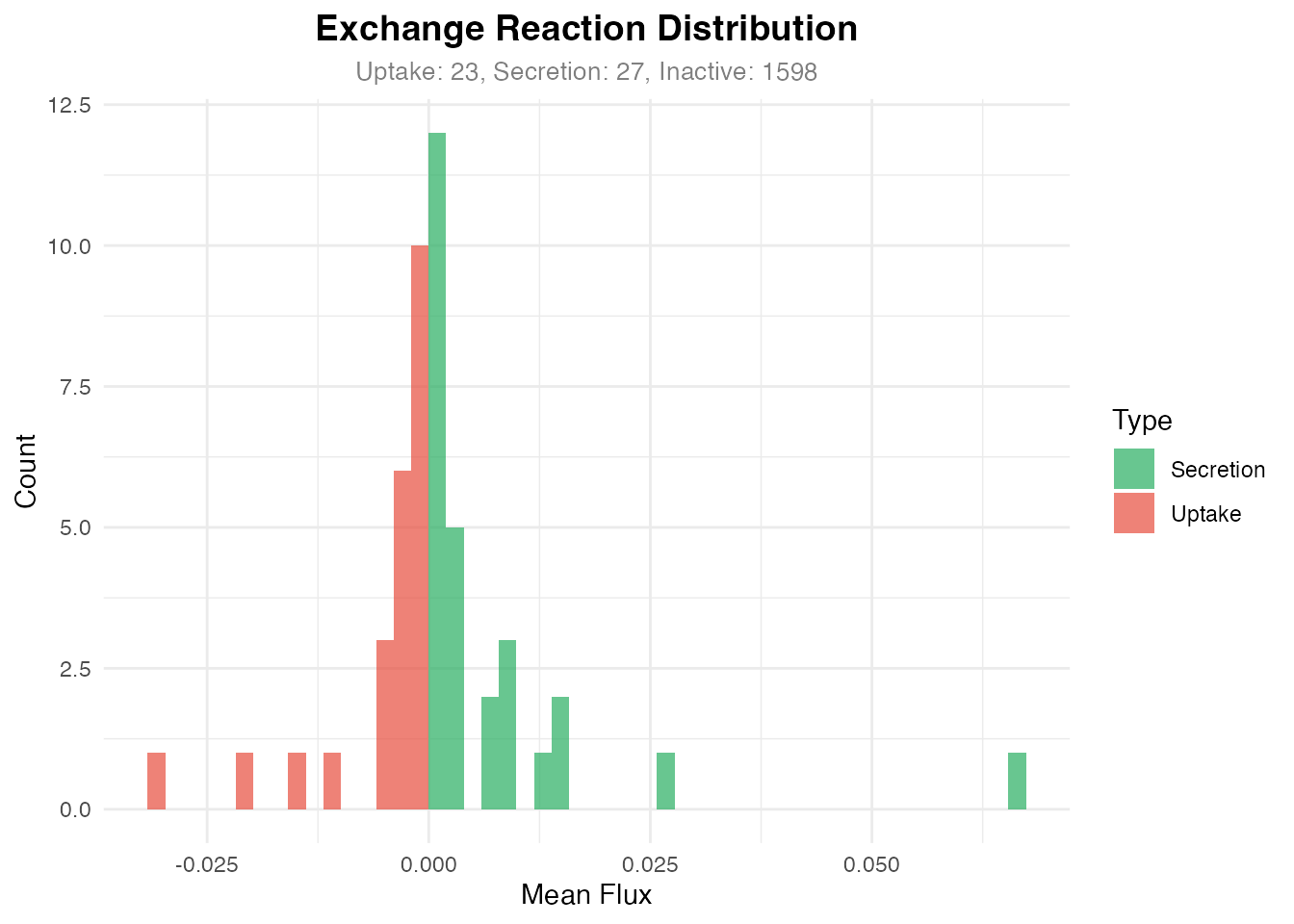
Distribution of uptake vs secretion reactions
Summary Statistics
cat("========================================\n")
#> ========================================
cat("METAFLUX Analysis Summary\n")
#> METAFLUX Analysis Summary
cat("========================================\n\n")
#> ========================================

cat("Input Data:\n")
#> Input Data:
cat(sprintf("  - Genes: %d\n", nrow(bulk_test_example)))
#>   - Genes: 58581
cat(sprintf("  - Samples: %d\n", ncol(bulk_test_example)))
#>   - Samples: 5

cat("\nOutput:\n")
#>
#> Output:
cat(sprintf("  - Reactions analyzed: %d\n", nrow(flux)))
#>   - Reactions analyzed: 13082
cat(sprintf("  - Flux range: [%.4f, %.4f]\n", min(flux), max(flux)))
#>   - Flux range: [-0.0840, 0.0841]

cat("\nKey Metabolites (mean flux):\n")
#>
#> Key Metabolites (mean flux):
for (met in names(key_rxns)) {
  val <- mean(flux[key_rxns[met], ])
  cat(sprintf("  - %s: %.4f\n", met, val))
}
#>   - Glucose: -0.0052
#>   - Lactate: 0.0020
#>   - Glutamine: -0.0015
#>   - Pyruvate: 0.0038
Session Information
sessionInfo()
#> R version 4.4.0 (2024-04-24)
#> Platform: aarch64-apple-darwin20
#> Running under: macOS 15.6.1
#>
#> Matrix products: default
#> BLAS:   /Library/Frameworks/R.framework/Versions/4.4-arm64/Resources/lib/libRblas.0.dylib
#> LAPACK: /Library/Frameworks/R.framework/Versions/4.4-arm64/Resources/lib/libRlapack.dylib;  LAPACK version 3.12.0
#>
#> locale:
#> [1] C
#>
#> time zone: Asia/Shanghai
#> tzcode source: internal
#>
#> attached base packages:
#> [1] stats     graphics  grDevices utils     datasets  methods   base
#>
#> other attached packages:
#> [1] ggplot2_4.0.1  METAFLUX_2.2.0
#>
#> loaded via a namespace (and not attached):
#>   [1] deldir_2.0-4           pbapply_1.7-4          gridExtra_2.3
#>   [4] rlang_1.1.7            magrittr_2.0.4         RcppAnnoy_0.0.23
#>   [7] otel_0.2.0             spatstat.geom_3.6-1    matrixStats_1.5.0
#>  [10] ggridges_0.5.7         compiler_4.4.0         png_0.1-8
#>  [13] systemfonts_1.3.1      vctrs_0.7.0            reshape2_1.4.5
#>  [16] stringr_1.6.0          pkgconfig_2.0.3        fastmap_1.2.0
#>  [19] labeling_0.4.3         promises_1.5.0         rmarkdown_2.30
#>  [22] ragg_1.5.0             purrr_1.2.1            xfun_0.56
#>  [25] cachem_1.1.0           jsonlite_2.0.0         goftest_1.2-3
#>  [28] later_1.4.5            spatstat.utils_3.2-1   irlba_2.3.5.1
#>  [31] parallel_4.4.0         cluster_2.1.8.1        R6_2.6.1
#>  [34] ica_1.0-3              spatstat.data_3.1-9    bslib_0.9.0
#>  [37] stringi_1.8.7          RColorBrewer_1.1-3     reticulate_1.44.1
#>  [40] spatstat.univar_3.1-6  parallelly_1.46.1      lmtest_0.9-40
#>  [43] jquerylib_0.1.4        scattermore_1.2        iterators_1.0.14
#>  [46] Rcpp_1.1.1             knitr_1.51             tensor_1.5.1
#>  [49] future.apply_1.20.1    zoo_1.8-15             sctransform_0.4.3
#>  [52] httpuv_1.6.16          Matrix_1.7-4           splines_4.4.0
#>  [55] igraph_2.2.1           tidyselect_1.2.1       abind_1.4-8
#>  [58] dichromat_2.0-0.1      yaml_2.3.12            doParallel_1.0.17
#>  [61] spatstat.random_3.4-3  spatstat.explore_3.6-0 codetools_0.2-20
#>  [64] miniUI_0.1.2           listenv_0.10.0         plyr_1.8.9
#>  [67] lattice_0.22-7         tibble_3.3.1           withr_3.0.2
#>  [70] shiny_1.12.1           S7_0.2.1               ROCR_1.0-11
#>  [73] evaluate_1.0.5         Rtsne_0.17             future_1.69.0
#>  [76] desc_1.4.3             survival_3.8-3         polyclip_1.10-7
#>  [79] fitdistrplus_1.2-4     osqp_0.6.3.3           pillar_1.11.1
#>  [82] Seurat_4.4.0           KernSmooth_2.23-26     foreach_1.5.2
#>  [85] plotly_4.11.0          generics_0.1.4         sp_2.2-0
#>  [88] scales_1.4.0           globals_0.18.0         xtable_1.8-4
#>  [91] glue_1.8.0             lazyeval_0.2.2         tools_4.4.0
#>  [94] data.table_1.18.0      RANN_2.6.2             fs_1.6.6
#>  [97] leiden_0.4.3.1         cowplot_1.2.0          grid_4.4.0
#> [100] tidyr_1.3.2            nlme_3.1-168           patchwork_1.3.2
#> [103] cli_3.6.5              spatstat.sparse_3.1-0  textshaping_1.0.4
#> [106] viridisLite_0.4.2      dplyr_1.1.4            uwot_0.2.4
#> [109] gtable_0.3.6           sass_0.4.10            digest_0.6.39
#> [112] progressr_0.18.0       ggrepel_0.9.6          htmlwidgets_1.6.4
#> [115] SeuratObject_4.1.4     farver_2.1.2           htmltools_0.5.9
#> [118] pkgdown_2.1.3          lifecycle_1.0.5        httr_1.4.7
#> [121] mime_0.13              MASS_7.3-65