Intercellular Communication Analysis with OmnipathR

Zaoqu Liu

Department of Interventional Radiology, The First Affiliated Hospital of Zhengzhou University
liuzaoqu@163.com

Dénes Türei

turei.denes@gmail.com

Julio Saez-Rodriguez

Institute for Computational Biomedicine, Heidelberg University
Source: vignettes/intercell_communication.Rmd

intercell_communication.Rmd

1 Introduction

Cell-cell communication is fundamental to multicellular organism function, coordinating processes from development to immune response. OmnipathR provides comprehensive access to ligand-receptor interactions and intercellular communication annotations, enabling systematic analysis of cellular crosstalk.

1.1 Biological Context

Intercellular signaling involves:

Ligands: Secreted or membrane-bound signaling molecules
Receptors: Cell surface proteins that receive signals
Downstream signaling: Intracellular cascades triggered by receptor activation

┌─────────────────┐                    ┌─────────────────┐
│   Sender Cell   │                    │  Receiver Cell  │
│                 │                    │                 │
│  ┌───────────┐  │    Ligand          │  ┌───────────┐  │
│  │  Ligand   │──┼───────────────────►│  │ Receptor  │  │
│  │  Gene     │  │                    │  │           │  │
│  └───────────┘  │                    │  └─────┬─────┘  │
│                 │                    │        │        │
│                 │                    │        ▼        │
│                 │                    │  ┌───────────┐  │
│                 │                    │  │ Signaling │  │
│                 │                    │  │  Cascade  │  │
│                 │                    │  └───────────┘  │
└─────────────────┘                    └─────────────────┘

2 Setup

library(OmnipathR)
library(dplyr)
library(tidyr)
library(ggplot2)

3 Intercellular Communication Database

3.1 Overview of Intercell Categories

OmnipathR organizes intercellular communication roles into a hierarchical system:

# Get all intercell categories
categories <- intercell_categories()

# View category summary
cat("Total categories:", length(categories), "\n")
#> Total categories: 833

# Show main categories
cat("\nSample categories:\n")
#> 
#> Sample categories:
head(categories, 20)
#>  [1] "transmembrane"                 "transmembrane_phobius"        
#>  [3] "transmembrane_sosui"           "transmembrane_tmhmm"          
#>  [5] "transmembrane_predicted"       "lhfpl"                        
#>  [7] "peripheral"                    "plasma_membrane"              
#>  [9] "basolateral_cell_membrane"     "basal_cell_membrane"          
#> [11] "apical_cell_membrane"          "apicolateral_cell_membrane"   
#> [13] "lateral_cell_membrane"         "plasma_membrane_transmembrane"
#> [15] "lhfpl_plasma_membrane"         "plasma_membrane_regulator"    
#> [17] "plasma_membrane_peripheral"    "secreted"                     
#> [19] "bpi_fold_containing"           "histatin"

3.2 Category Types

Category	Description	Examples
Ligand	Secreted signaling molecules	Cytokines, growth factors
Receptor	Signal-receiving proteins	RTKs, GPCRs
ECM	Extracellular matrix components	Collagens, laminins
Adhesion	Cell adhesion molecules	Integrins, cadherins
Transporter	Membrane transporters	Ion channels, ABC transporters

4 Retrieving Intercell Data

4.1 Basic Intercell Annotations

# Get intercell annotations
intercell_data <- intercell()

cat("Total intercell records:", nrow(intercell_data), "\n")
#> Total intercell records: 388239

# Summary of categories
category_counts <- intercell_data %>%
    count(category, sort = TRUE)

head(category_counts, 15)
#> # A tibble: 15 x 2
#>    category                           n
#>    <chr>                          <int>
#>  1 intracellular                 162594
#>  2 transmembrane                  51903
#>  3 receptor                       35316
#>  4 plasma_membrane                15891
#>  5 secreted                       15858
#>  6 ligand                         15698
#>  7 ecm                            10459
#>  8 cell_surface                   10438
#>  9 extracellular                   9443
#> 10 plasma_membrane_transmembrane   7902
#> 11 cell_adhesion                   4845
#> 12 gpcr                            4370
#> 13 adhesion                        2964
#> 14 cell_surface_ligand             2664
#> 15 ion_channel                     2160

4.2 Category Distribution Visualization

# Visualize top categories
top_categories <- category_counts %>% head(12)

ggplot(top_categories, aes(x = reorder(category, n), y = n, fill = category)) +
    geom_col(alpha = 0.8) +
    coord_flip() +
    scale_fill_viridis_d(guide = "none") +
    labs(
        title = "Intercellular Communication Categories",
        subtitle = "Number of annotated proteins per category",
        x = "Category",
        y = "Number of Proteins"
    ) +
    theme_minimal() +
    theme(
        plot.title = element_text(face = "bold", size = 14),
        axis.text.y = element_text(size = 9)
    )

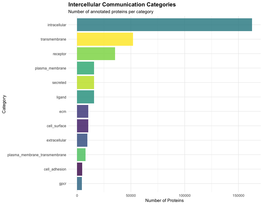
Figure 4.1: Distribution of proteins across major intercellular communication categories.

5 Ligand-Receptor Interactions

5.1 Curated Ligand-Receptor Database

# Get curated ligand-receptor interactions
lr_interactions <- tryCatch(
    curated_ligand_receptor_interactions(),
    error = function(e) {
        message("Note: Unable to fetch data from OmniPath server: ", e$message)
        # Return sample data structure for demonstration
        data.frame(
            source_genesymbol = c("TGFB1", "WNT3A", "FGF2", "EGF", "VEGFA"),
            target_genesymbol = c("TGFBR1", "FZD1", "FGFR1", "EGFR", "KDR"),
            sources = rep("CellPhoneDB", 5)
        )
    }
)

cat("Total L-R pairs:", nrow(lr_interactions), "\n")
#> Total L-R pairs: 6744

# View example interactions
lr_interactions %>%
    select(source_genesymbol, target_genesymbol, sources) %>%
    head(10)
#> # A tibble: 10 x 3
#>    source_genesymbol target_genesymbol sources                                  
#>    <chr>             <chr>             <chr>                                    
#>  1 JAG2              NOTCH1            Baccin2019;CellCall;CellChatDB;CellPhone~
#>  2 IL22              IL10RB            CellCall;CellTalkDB;Fantom5_LRdb;Guide2P~
#>  3 EPO               EPOR              Baccin2019;BioGRID;CellCall;CellChatDB;C~
#>  4 CXCL16            CXCR6             Baccin2019;CellCall;CellChatDB;CellPhone~
#>  5 KITLG             KIT               Baccin2019;BioGRID;CancerCellMap;CellCal~
#>  6 CXCL9             CXCR3             Baccin2019;BioGRID;CellCall;CellChatDB;C~
#>  7 CCL5              CCR5              BioGRID;CellCall;CellChatDB;CellPhoneDB;~
#>  8 CCL8              CCR5              Baccin2019;CellCall;CellPhoneDB;CellPhon~
#>  9 CCL4              CCR5              Baccin2019;CellCall;CellChatDB;CellPhone~
#> 10 IL6               IL6ST             Baccin2019;CellCall;CellTalkDB;DIP;DLRP_~

5.2 Ligand-Receptor Network Statistics

# Count interactions per ligand
ligand_counts <- lr_interactions %>%
    count(source_genesymbol, name = "n_receptors", sort = TRUE) %>%
    head(15) %>%
    mutate(type = "Ligand")

# Count interactions per receptor  
receptor_counts <- lr_interactions %>%
    count(target_genesymbol, name = "n_ligands", sort = TRUE) %>%
    head(15) %>%
    mutate(type = "Receptor")

# Combine for visualization
combined_counts <- bind_rows(
    ligand_counts %>% rename(gene = source_genesymbol, count = n_receptors),
    receptor_counts %>% rename(gene = target_genesymbol, count = n_ligands)
)

ggplot(combined_counts, aes(x = reorder(gene, count), y = count, fill = type)) +
    geom_col(alpha = 0.8) +
    coord_flip() +
    facet_wrap(~type, scales = "free_y") +
    scale_fill_manual(values = c("Ligand" = "#E74C3C", "Receptor" = "#3498DB")) +
    labs(
        title = "Top Ligands and Receptors",
        subtitle = "Ranked by number of interaction partners",
        x = "Gene",
        y = "Number of Partners"
    ) +
    theme_minimal() +
    theme(
        plot.title = element_text(face = "bold"),
        legend.position = "none",
        strip.text = element_text(face = "bold")
    )

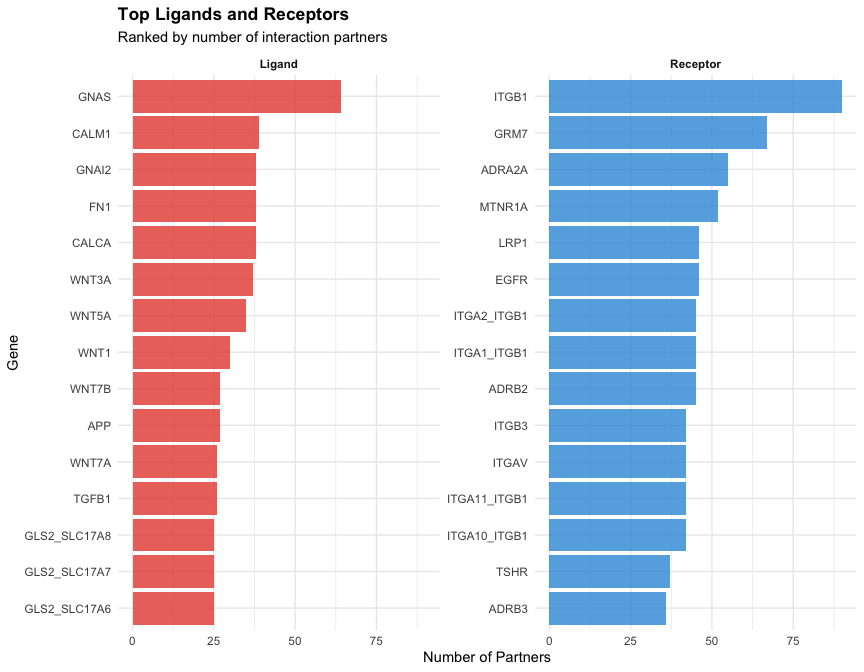
Figure 5.1: Top ligands and receptors by number of interaction partners in the curated database.

6 Analysis Workflows

6.1 Ligand Classification

# Get all ligands
ligands <- intercell_data %>%
    filter(category == "ligand" | grepl("ligand", category)) %>%
    pull(genesymbol) %>%
    unique()

cat("Total ligands:", length(ligands), "\n")
#> Total ligands: 2932

# Show sample ligands
head(ligands, 20)
#>  [1] "CXCL3"   "SEMA3B"  "NID1"    "IL3"     "PF4"     "LTA"     "C1QTNF1"
#>  [8] "VEGFA"   "PLG"     "IL1RN"   "CXCL2"   "WNT4"    "GAL"     "FGF3"   
#> [15] "ANGPTL3" "HP"      "DEFB1"   "EFNB2"   "IL17A"   "IFNA8"

6.2 Receptor Classification

# Get receptor annotations
receptors <- intercell_data %>%
    filter(grepl("receptor", category, ignore.case = TRUE))

# Classify receptors by category
receptor_types <- receptors %>%
    count(category, sort = TRUE) %>%
    head(10)

ggplot(receptor_types, aes(x = reorder(category, n), y = n, fill = category)) +
    geom_col(alpha = 0.8) +
    coord_flip() +
    scale_fill_viridis_d(guide = "none") +
    labs(
        title = "Receptor Classification",
        subtitle = "Distribution across receptor subcategories",
        x = "Receptor Category",
        y = "Number of Proteins"
    ) +
    theme_minimal() +
    theme(
        plot.title = element_text(face = "bold"),
        axis.text.y = element_text(size = 9)
    )

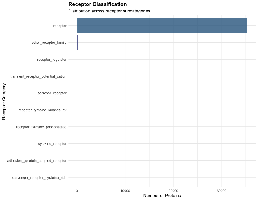
Figure 6.1: Classification of receptors by subcategory showing the diversity of receptor types in the database.

7 Resource Comparison

# Analyze resources contributing to L-R interactions
if("sources" %in% colnames(lr_interactions)) {
    resource_counts <- lr_interactions %>%
        separate_rows(sources, sep = ";") %>%
        count(sources, sort = TRUE) %>%
        head(12)
    
    ggplot(resource_counts, aes(x = reorder(sources, n), y = n)) +
        geom_col(fill = "#007B7F", alpha = 0.8) +
        coord_flip() +
        labs(
            title = "Ligand-Receptor Resources",
            subtitle = "Number of interactions per resource",
            x = "Resource",
            y = "Interactions"
        ) +
        theme_minimal() +
        theme(plot.title = element_text(face = "bold"))
}

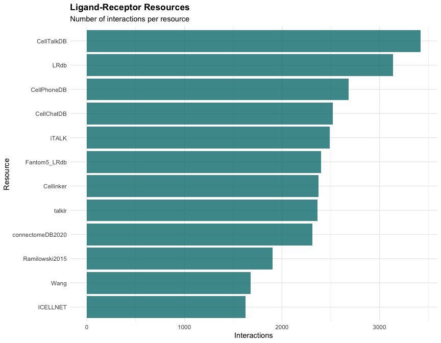
Figure 7.1: Comparison of ligand-receptor interaction coverage across different resources integrated in OmniPath.

8 Session Information

sessionInfo()
#> R version 4.4.0 (2024-04-24)
#> Platform: aarch64-apple-darwin20
#> Running under: macOS 15.6.1
#> 
#> Matrix products: default
#> BLAS:   /Library/Frameworks/R.framework/Versions/4.4-arm64/Resources/lib/libRblas.0.dylib 
#> LAPACK: /Library/Frameworks/R.framework/Versions/4.4-arm64/Resources/lib/libRlapack.dylib;  LAPACK version 3.12.0
#> 
#> locale:
#> [1] C
#> 
#> time zone: Asia/Shanghai
#> tzcode source: internal
#> 
#> attached base packages:
#> [1] stats     graphics  grDevices utils     datasets  methods   base     
#> 
#> other attached packages:
#> [1] ggplot2_4.0.1    tidyr_1.3.2      dplyr_1.1.4      OmnipathR_3.19.1
#> 
#> loaded via a namespace (and not attached):
#>  [1] gtable_0.3.6       xfun_0.56          bslib_0.9.0        httr2_1.2.2       
#>  [5] htmlwidgets_1.6.4  websocket_1.4.4    processx_3.8.6     tzdb_0.5.0        
#>  [9] vctrs_0.7.0        tools_4.4.0        ps_1.9.1           generics_0.1.4    
#> [13] curl_7.0.0         tibble_3.3.1       RSQLite_2.4.5      blob_1.2.4        
#> [17] pkgconfig_2.0.3    R.oo_1.27.1        checkmate_2.3.3    RColorBrewer_1.1-3
#> [21] S7_0.2.1           readxl_1.4.5       lifecycle_1.0.5    farver_2.1.2      
#> [25] compiler_4.4.0     stringr_1.6.0      progress_1.2.3     chromote_0.5.1    
#> [29] htmltools_0.5.9    sass_0.4.10        yaml_2.3.12        later_1.4.5       
#> [33] pillar_1.11.1      crayon_1.5.3       jquerylib_0.1.4    R.utils_2.13.0    
#> [37] cachem_1.1.0       sessioninfo_1.2.3  zip_2.3.3          tidyselect_1.2.1  
#> [41] rvest_1.0.5        digest_0.6.39      stringi_1.8.7      purrr_1.2.1       
#> [45] bookdown_0.44      labeling_0.4.3     grid_4.4.0         fastmap_1.2.0     
#> [49] cli_3.6.5          logger_0.4.1       magrittr_2.0.4     utf8_1.2.6        
#> [53] dichromat_2.0-0.1  XML_3.99-0.20      withr_3.0.2        readr_2.1.6       
#> [57] scales_1.4.0       prettyunits_1.2.0  promises_1.5.0     backports_1.5.0   
#> [61] rappdirs_0.3.4     bit64_4.6.0-1      lubridate_1.9.4    timechange_0.3.0  
#> [65] rmarkdown_2.30     httr_1.4.7         igraph_2.2.1       bit_4.6.0         
#> [69] otel_0.2.0         cellranger_1.1.0   R.methodsS3_1.8.2  hms_1.1.4         
#> [73] memoise_2.0.1      evaluate_1.0.5     knitr_1.51         tcltk_4.4.0       
#> [77] viridisLite_0.4.2  rlang_1.1.7        Rcpp_1.1.1         glue_1.8.0        
#> [81] DBI_1.2.3          selectr_0.5-1      xml2_1.5.2         vroom_1.6.7       
#> [85] jsonlite_2.0.0     R6_2.6.1           fs_1.6.6

9 References

Türei D, et al. Integrated intra- and intercellular signaling knowledge for multicellular omics analysis. Molecular Systems Biology 2021;17:e9923.
Efremova M, et al. CellPhoneDB: inferring cell–cell communication from combined expression of multi-subunit ligand–receptor complexes. Nature Protocols 2020;15:1484-1506.
Ramilowski JA, et al. A draft network of ligand–receptor-mediated multicellular signalling in human. Nature Communications 2015;6:7866.