SVG: A Comprehensive R Package for Spatially Variable Gene Detection

Zaoqu Liu

2026-01-23

Abstract

Spatial transcriptomics has emerged as a transformative technology in modern biology, enabling the simultaneous measurement of gene expression and spatial localization within tissues. A fundamental analytical challenge is the identification of Spatially Variable Genes (SVGs) — genes exhibiting non-random spatial expression patterns that may reflect underlying biological structures or gradients. This vignette provides a comprehensive introduction to the SVG package, which implements six state-of-the-art SVG detection methods within a unified computational framework. We present the mathematical foundations of each method, demonstrate their application through extensive examples, compare their performance characteristics, and provide practical guidelines for method selection in various experimental contexts.

Keywords: Spatial transcriptomics, Spatially variable genes, Moran’s I, Gaussian processes, Spatial statistics, R package

---

Introduction

Background and Motivation

The emergence of spatial transcriptomics technologies, including 10x Genomics Visium, Slide-seq, MERFISH, and seqFISH, has revolutionized our understanding of tissue architecture by preserving the spatial context of gene expression measurements. Unlike single-cell RNA sequencing, which dissociates cells from their native environment, spatial transcriptomics maintains the positional information of transcripts, enabling the study of:

• Tissue organization and cellular neighborhoods
• Spatial gradients in developmental processes
• Cell-cell communication and signaling microenvironments
• Pathological patterns in disease contexts

A critical first step in spatial transcriptomics analysis is identifying genes whose expression patterns exhibit significant spatial structure — the so-called Spatially Variable Genes (SVGs). These genes serve as:

1. Markers for distinct tissue regions or cell populations
2. Candidates for spatial signaling pathways
3. Features for downstream clustering and trajectory analysis

Package Overview

The SVG package provides a unified, high-performance implementation of multiple SVG detection methods:

Method	Statistical Framework	Key Features
MERINGUE	Moran’s I with spatial networks	Network-based, interpretable statistic
binSpect	Fisher’s exact test	Fast, robust to outliers
SPARK-X	Kernel-based association	Multi-scale pattern detection
Seurat	Moran’s I with distance weights	Compatible with Seurat workflow
nnSVG	Gaussian processes (NNGP)	Full statistical model, effect size
MarkVario	Mark variogram	Non-parametric spatial statistics

Each method has distinct theoretical foundations and practical trade-offs, which we systematically explore in this vignette.

---

Mathematical Foundations

Understanding the mathematical principles underlying SVG detection methods is essential for appropriate method selection and result interpretation. This section provides rigorous derivations of the key statistical frameworks.

Spatial Autocorrelation: Moran’s I Statistic

Definition and Intuition

Moran’s I is a classical measure of global spatial autocorrelation, introduced by Patrick Moran in 1950. For gene expression values $\mathbf{x} = (x_1, x_2, \ldots, x_n)^T$ measured at $n$ spatial locations with coordinates $\mathbf{s}_1, \mathbf{s}_2, \ldots, \mathbf{s}_n$, Moran’s I is defined as:

$$I = \frac{n}{\sum_{i=1}^{n}\sum_{j=1}^{n} w_{ij}} \cdot \frac{\sum_{i=1}^{n}\sum_{j=1}^{n} w_{ij}(x_i - \bar{x})(x_j - \bar{x})}{\sum_{i=1}^{n}(x_i - \bar{x})^2}$$

where:

• $w_{ij}$ is the spatial weight between locations $i$ and $j$
• $\bar{x} = \frac{1}{n}\sum_{i=1}^{n} x_i$ is the sample mean
• $\mathbf{W} = [w_{ij}]$ is the spatial weights matrix

Interpretation:

• $I \approx 1$: Strong positive autocorrelation (similar values cluster)
• $I \approx -1$: Strong negative autocorrelation (dissimilar values neighbor each other)
• $I \approx E[I]$: Random spatial pattern

Statistical Inference

Under the null hypothesis $H_0$ of complete spatial randomness (CSR), the expected value of Moran’s I is:

$$E[I] = -\frac{1}{n-1}$$

The variance under the randomization assumption is given by:

$$\text{Var}[I] = \frac{nS_1 - S_2n + 3S_0^2}{S_0^2(n^2-1)} - E[I]^2$$

where:

• $S_0 = \sum_{i}\sum_{j} w_{ij}$ (sum of all weights)
• $S_1 = \frac{1}{2}\sum_{i}\sum_{j}(w_{ij} + w_{ji})^2$
• $S_2 = \sum_{k}(\sum_{j} w_{kj} + \sum_{i} w_{ik})^2$

The standardized test statistic follows an asymptotic normal distribution:

$$Z = \frac{I - E[I]}{\sqrt{\text{Var}[I]}} \xrightarrow{d} N(0, 1)$$

Spatial Weights Specifications

The choice of spatial weights matrix $\mathbf{W}$ is crucial and method-specific:

Binary Adjacency (MERINGUE): $$w_{ij} = \begin{cases} 1 & \text{if } i \text{ and } j \text{ are neighbors} \\ 0 & \text{otherwise} \end{cases}$$

Neighbors can be defined via: - Delaunay triangulation: Natural neighborhood based on Voronoi tessellation - K-nearest neighbors (KNN): Fixed number of closest points

Inverse Distance (Seurat): $$w_{ij} = \frac{1}{d_{ij}^2}$$

where $d_{ij} = \|\mathbf{s}_i - \mathbf{s}_j\|_2$ is the Euclidean distance.

Gaussian Kernel: $$w_{ij} = \exp\left(-\frac{d_{ij}^2}{2h^2}\right)$$

where $h$ is the bandwidth parameter.

Kernel-Based Association Tests: SPARK-X

Variance Component Score Test

SPARK-X employs a kernel-based framework to detect spatial patterns through variance component testing. For centered gene expression $\mathbf{y} = \mathbf{x} - \bar{x}\mathbf{1}$, the test statistic is:

$$T = n \cdot \frac{\mathbf{y}^T \mathbf{K} \mathbf{y}}{\|\mathbf{y}\|^2}$$

where $\mathbf{K}$ is a kernel matrix capturing spatial similarity.

Multiple Kernel Types

SPARK-X employs three classes of kernels to detect diverse spatial patterns:

1. Linear (Projection) Kernel: $$\mathbf{K}_{\text{linear}} = \mathbf{X}(\mathbf{X}^T\mathbf{X})^{-1}\mathbf{X}^T$$

Detects linear gradients and directional trends.

2. Gaussian RBF Kernels (5 scales): $$K_{\text{Gaussian}}^{(l)}(i,j) = \exp\left(-\frac{d_{ij}^2}{2h_l^2}\right), \quad l = 1, \ldots, 5$$

where bandwidths $h_l$ correspond to the 20th, 40th, 60th, 80th, and 100th percentiles of pairwise distances. These detect localized hotspots of varying sizes.

3. Cosine/Periodic Kernels (5 scales): $$K_{\text{Cosine}}^{(l)}(i,j) = \cos\left(\frac{2\pi d_{ij}}{h_l}\right)$$

Detect periodic or oscillating spatial patterns.

P-value Computation and Combination

For each kernel, p-values are computed using Davies’ method for quadratic forms in normal variables. The distribution of $T$ under the null follows:

$$T \sim \sum_{k=1}^{r} \lambda_k \chi^2_{1,k}$$

where $\lambda_k$ are eigenvalues of the centered kernel matrix.

P-values from all 11 kernels are combined using the Aggregated Cauchy Association Test (ACAT):

$$T_{\text{ACAT}} = \sum_{l=1}^{11} w_l \tan\left[(0.5 - p_l)\pi\right]$$

The combined p-value is then:

$$p_{\text{combined}} = \frac{1}{2} - \frac{\arctan(T_{\text{ACAT}})}{\pi}$$

ACAT is robust to dependency among tests and maintains correct type I error.

Binary Spatial Enrichment: binSpect

Methodology

The binSpect method from Giotto converts continuous expression into binary categories and tests for spatial enrichment using contingency tables.

Step 1: Expression Binarization

For gene $g$, expression values are classified as “high” or “low” using k-means clustering ($k=2$):

$$b_i = \begin{cases} 1 & \text{if } x_i \in \text{high-expression cluster} \\ 0 & \text{otherwise} \end{cases}$$

Step 2: Spatial Contingency Table

For all pairs of neighboring spots $(i, j)$ in the spatial network:

	Neighbor High	Neighbor Low
Spot High	$n_{11}$	$n_{10}$
Spot Low	$n_{01}$	$n_{00}$

Step 3: Fisher’s Exact Test

The odds ratio quantifies spatial enrichment:

$$\text{OR} = \frac{n_{11} \cdot n_{00}}{n_{10} \cdot n_{01}}$$

• $\text{OR} > 1$: High-expressing cells cluster together
• $\text{OR} < 1$: High-expressing cells avoid each other
• $\text{OR} = 1$: Random spatial distribution

Fisher’s exact test provides exact p-values for the null hypothesis $H_0: \text{OR} = 1$.

Nearest-Neighbor Gaussian Processes: nnSVG

Full Statistical Model

nnSVG provides the most complete statistical framework by modeling spatial correlation through Gaussian processes:

$$\mathbf{y} = \mathbf{X}\boldsymbol{\beta} + \mathbf{w}(\mathbf{s}) + \boldsymbol{\epsilon}$$

where:

• $\mathbf{y}$ is the $n \times 1$ expression vector
• $\mathbf{X}$ is the design matrix (covariates)
• $\boldsymbol{\beta}$ is the coefficient vector
• $\mathbf{w}(\mathbf{s}) \sim GP(\mathbf{0}, \sigma^2 \mathbf{C}_\phi)$ is the spatial random effect
• $\boldsymbol{\epsilon} \sim N(\mathbf{0}, \tau^2 \mathbf{I})$ is the nugget (non-spatial variance)

Covariance Function

The spatial covariance is typically modeled using the exponential function:

$$C_\phi(d) = \exp\left(-\frac{d}{\phi}\right)$$

where $\phi$ is the range parameter controlling spatial decay.

NNGP Approximation

Full GP has $O(n^3)$ complexity. The Nearest-Neighbor Gaussian Process approximates the likelihood using only $m$ nearest neighbors:

$$p(\mathbf{y}) \approx \prod_{i=1}^{n} p(y_i | y_{\mathcal{N}(i)})$$

This reduces complexity to $O(n \cdot m^3)$, enabling scalable computation.

Likelihood Ratio Test

SVGs are identified via likelihood ratio test:

$$\text{LR} = -2 \left[\log L(\text{null}) - \log L(\text{spatial})\right]$$

Under $H_0$ (no spatial effect), $\text{LR} \sim \chi^2_2$.

Effect Size: Proportion of Spatial Variance

The proportion of variance explained by spatial structure:

$$\text{prop\_sv} = \frac{\hat{\sigma}^2}{\hat{\sigma}^2 + \hat{\tau}^2}$$

• $\text{prop\_sv} \to 1$: Strong spatial pattern
• $\text{prop\_sv} \to 0$: Little spatial structure

---

Installation and Setup

# Install from GitHub
devtools::install_github("Zaoqu-Liu/SVG")

# Install all optional dependencies
install.packages(c("geometry", "RANN", "BRISC", "CompQuadForm", 
                   "spatstat.geom", "spatstat.explore"))

# Load the SVG package
library(SVG)

# Load the built-in example dataset
data(example_svg_data)

# Display dataset structure
cat("Dataset components:\n")
#> Dataset components:
names(example_svg_data)
#> [1] "counts"         "logcounts"      "spatial_coords" "gene_info"     
#> [5] "params"

---

Data Description and Visualization

Simulated Spatial Transcriptomics Data

The example_svg_data contains simulated spatial transcriptomics data designed to benchmark SVG detection methods:

# Extract components
expr_counts <- example_svg_data$counts        # Raw counts
expr_log <- example_svg_data$logcounts        # Log-normalized
coords <- example_svg_data$spatial_coords     # Spatial coordinates
gene_info <- example_svg_data$gene_info       # Gene metadata

cat("Data Dimensions:\n")
#> Data Dimensions:
cat("  Number of spots:", ncol(expr_counts), "\n")
#>   Number of spots: 500
cat("  Number of genes:", nrow(expr_counts), "\n")
#>   Number of genes: 200
cat("  True SVGs:", sum(gene_info$is_svg), "\n")
#>   True SVGs: 50
cat("  Non-SVGs:", sum(!gene_info$is_svg), "\n")
#>   Non-SVGs: 150
cat("\nSpatial Pattern Types:\n")
#> 
#> Spatial Pattern Types:
print(table(gene_info$pattern_type))
#> 
#>  cluster gradient  hotspot     none periodic 
#>       11       13       13      150       13

Spatial Spot Layout

The spots are arranged in a hexagonal grid pattern, mimicking the 10x Genomics Visium platform:

par(mar = c(4, 4, 3, 2))
plot(coords[, 1], coords[, 2],
     pch = 19, cex = 0.9,
     col = adjustcolor("steelblue", alpha.f = 0.7),
     xlab = "X coordinate (μm)",
     ylab = "Y coordinate (μm)",
     main = "Spatial Spot Layout (Hexagonal Grid)",
     asp = 1)
grid(lty = 2, col = "gray80")

# Add spot count annotation
mtext(paste("n =", nrow(coords), "spots"), side = 3, line = 0.3, cex = 0.9)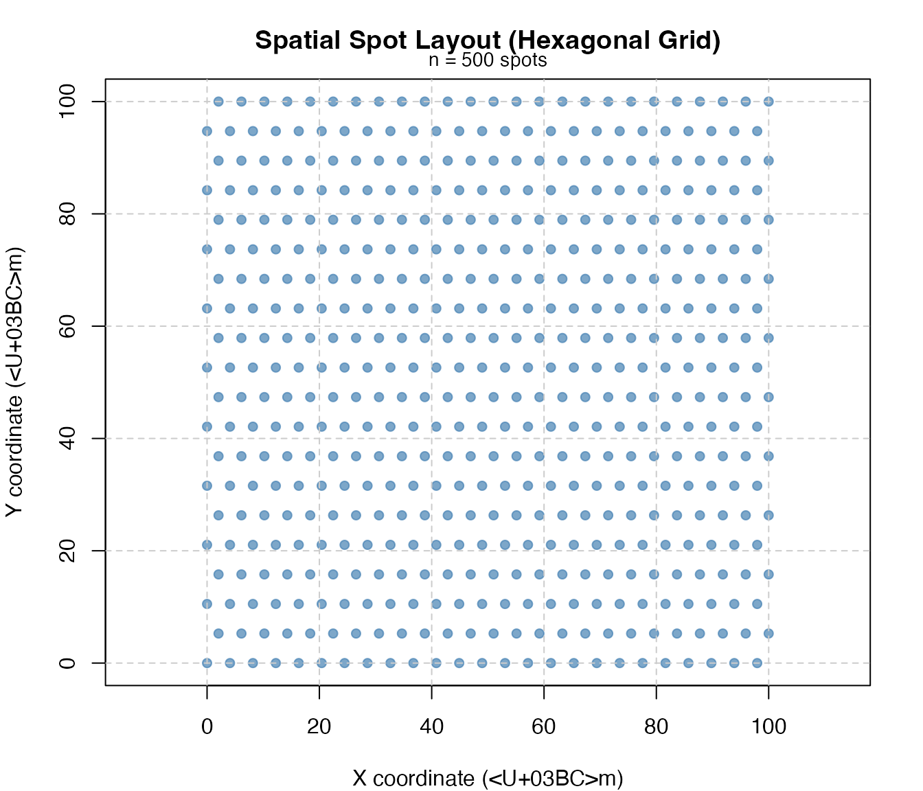

Gene Expression Distribution

par(mfrow = c(1, 2), mar = c(4, 4, 3, 1))

# Raw counts distribution
hist(log10(rowMeans(expr_counts) + 1), breaks = 30,
     col = "lightblue", border = "white",
     xlab = expression(log[10](Mean~Count + 1)),
     ylab = "Number of Genes",
     main = "Gene Expression Distribution")

# Spot library size
hist(log10(colSums(expr_counts)), breaks = 30,
     col = "lightgreen", border = "white",
     xlab = expression(log[10](Library~Size)),
     ylab = "Number of Spots",
     main = "Spot Library Size Distribution")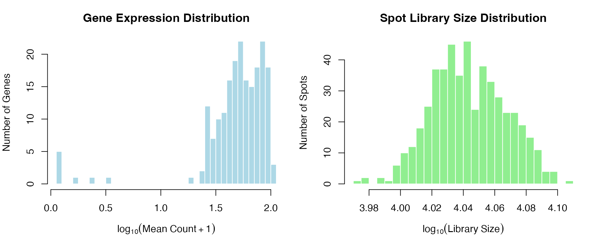

Spatial Expression Pattern Visualization

The simulated data contains four distinct spatial pattern types for SVGs:

# Define color palette for expression visualization
expr_colors <- function(x, pal = "RdYlBu") {
  x_scaled <- (x - min(x, na.rm = TRUE)) / (max(x, na.rm = TRUE) - min(x, na.rm = TRUE) + 1e-10)
  if (pal == "RdYlBu") {
    colors <- colorRampPalette(c("#313695", "#4575B4", "#74ADD1", "#ABD9E9", 
                                  "#E0F3F8", "#FFFFBF", "#FEE090", "#FDAE61", 
                                  "#F46D43", "#D73027", "#A50026"))(100)
  } else {
    colors <- colorRampPalette(c("navy", "white", "firebrick3"))(100)
  }
  colors[pmax(1, ceiling(x_scaled * 99) + 1)]
}

# Get example genes for each pattern type
pattern_types <- c("gradient", "hotspot", "periodic", "cluster")
pattern_genes <- sapply(pattern_types, function(pt) {
  which(gene_info$pattern_type == pt)[1]
})

# Get non-SVG example
non_svg_gene <- which(!gene_info$is_svg)[1]

par(mfrow = c(2, 3), mar = c(4, 4, 3, 1))

# Plot each pattern type
for (i in seq_along(pattern_types)) {
  gene_idx <- pattern_genes[i]
  gene_name <- rownames(expr_log)[gene_idx]
  gene_expr <- expr_log[gene_idx, ]
  
  plot(coords[, 1], coords[, 2],
       pch = 19, cex = 1.3,
       col = expr_colors(gene_expr),
       xlab = "X", ylab = "Y",
       main = paste0(gene_name, "\n(", pattern_types[i], " pattern)"),
       asp = 1)
}

# Plot non-SVG
gene_expr <- expr_log[non_svg_gene, ]
plot(coords[, 1], coords[, 2],
     pch = 19, cex = 1.3,
     col = expr_colors(gene_expr),
     xlab = "X", ylab = "Y",
     main = paste0(rownames(expr_log)[non_svg_gene], "\n(non-SVG, random)"),
     asp = 1)

# Add color legend
plot.new()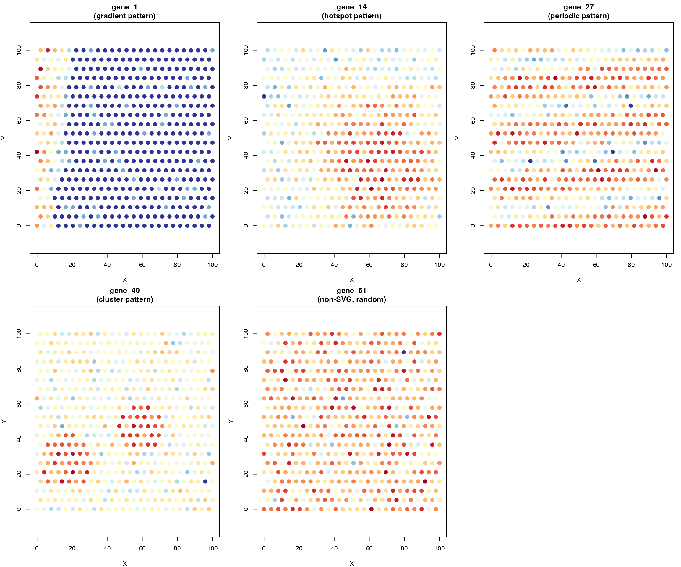

par(mar = c(1, 1, 1, 1))
legend_colors <- colorRampPalette(c("#313695", "#FFFFBF", "#A50026"))(100)
legend_image <- as.raster(matrix(rev(legend_colors), ncol = 1))
plot(c(0, 1), c(0, 1), type = "n", axes = FALSE, xlab = "", ylab = "")
text(0.5, 0.95, "Expression Level", cex = 1.2, font = 2)
rasterImage(legend_image, 0.3, 0.1, 0.7, 0.85)
text(0.75, 0.1, "Low", cex = 0.9)
text(0.75, 0.85, "High", cex = 0.9)

---

SVG Detection: Method-by-Method Tutorial

Method 1: MERINGUE (Moran’s I with Spatial Networks)

Algorithm Overview

MERINGUE computes Moran’s I statistic using a sparse spatial adjacency network, offering computational efficiency while maintaining statistical power.

Key Steps:

1. Construct spatial neighborhood network (Delaunay or KNN)
2. Compute Moran’s I for each gene
3. Calculate analytical p-values under normal approximation
4. Apply multiple testing correction

Running MERINGUE

# Run MERINGUE with KNN network
results_meringue <- CalSVG_MERINGUE(
  expr_matrix = expr_log,
  spatial_coords = coords,
  network_method = "knn",       # Network construction method
  k = 10,                       # Number of neighbors
  alternative = "greater",      # Test for positive autocorrelation
  adjust_method = "BH",         # Benjamini-Hochberg correction
  verbose = FALSE
)

# Display top SVGs
cat("Top 10 SVGs by MERINGUE:\n")
#> Top 10 SVGs by MERINGUE:
head(results_meringue[, c("gene", "observed", "expected", "z_score", "p.value", "p.adj")], 10)
#>       gene  observed     expected   z_score p.value p.adj
#> 1   gene_1 0.7667350 -0.002004008 39.717880       0     0
#> 2   gene_2 0.4929258 -0.002004008 25.686514       0     0
#> 3   gene_3 0.1744444 -0.002004008  9.287831       0     0
#> 4   gene_4 0.4593775 -0.002004008 23.759281       0     0
#> 5   gene_5 0.7236521 -0.002004008 37.422043       0     0
#> 6   gene_6 0.1587466 -0.002004008  8.496923       0     0
#> 7   gene_7 0.9056749 -0.002004008 46.670022       0     0
#> 8   gene_8 0.2925418 -0.002004008 15.388682       0     0
#> 9   gene_9 0.8262118 -0.002004008 42.721016       0     0
#> 10 gene_10 0.4378317 -0.002004008 22.658627       0     0

Visualizing MERINGUE Results

par(mfrow = c(1, 2), mar = c(4, 4, 3, 1))

# Moran's I distribution
hist(results_meringue$observed, breaks = 40,
     col = "steelblue", border = "white",
     xlab = "Moran's I",
     ylab = "Number of Genes",
     main = "Distribution of Moran's I Statistics")
abline(v = results_meringue$expected[1], col = "red", lwd = 2, lty = 2)
legend("topright", legend = "E[I] under null", col = "red", lty = 2, lwd = 2)

# P-value distribution
hist(results_meringue$p.value, breaks = 40,
     col = "coral", border = "white",
     xlab = "P-value",
     ylab = "Number of Genes",
     main = "P-value Distribution")
abline(v = 0.05, col = "darkred", lwd = 2, lty = 2)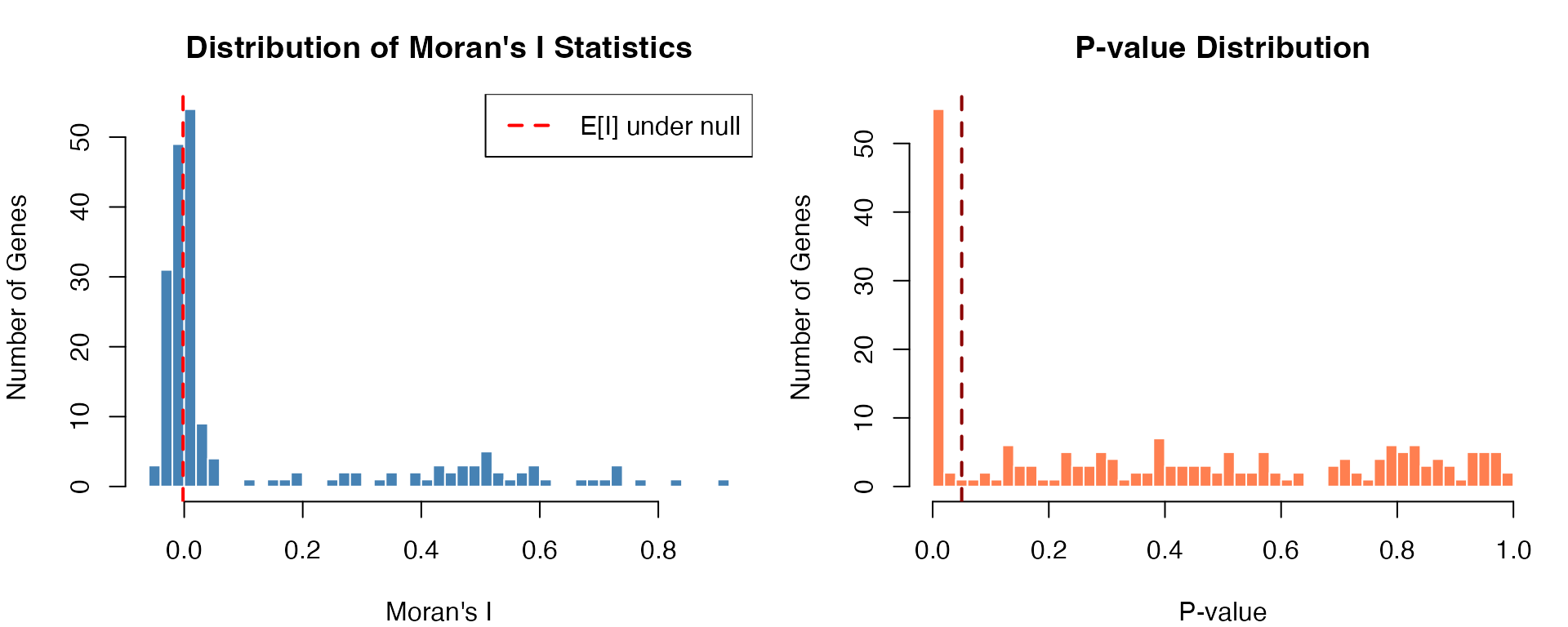

Method 2: binSpect (Binary Spatial Enrichment)

Algorithm Overview

binSpect converts continuous expression to binary categories and uses Fisher’s exact test to detect spatial clustering.

Key Steps:

1. Binarize gene expression (k-means or rank-based)
2. Build spatial neighborhood network
3. Construct contingency tables for neighbor pairs
4. Perform Fisher’s exact test for each gene

Running binSpect

# Run binSpect with k-means binarization
results_binspect <- CalSVG_binSpect(
  expr_matrix = expr_log,
  spatial_coords = coords,
  bin_method = "kmeans",        # Binarization method
  network_method = "delaunay",  # Network construction
  do_fisher_test = TRUE,        # Perform Fisher's test
  adjust_method = "fdr",        # FDR correction
  verbose = FALSE
)

# Display top SVGs
cat("Top 10 SVGs by binSpect:\n")
#> Top 10 SVGs by binSpect:
head(results_binspect[, c("gene", "estimate", "p.value", "p.adj", "score")], 10)
#>       gene  estimate       p.value         p.adj     score
#> 1   gene_7 239.82358 1.881408e-272 3.762816e-270 65166.186
#> 2   gene_9 352.47489 9.696440e-174 9.696440e-172 60982.874
#> 3   gene_1 320.18186 7.426544e-152 3.713272e-150 48388.833
#> 4  gene_41 102.16057 4.940292e-142 1.646764e-140 14435.927
#> 5  gene_42  50.21381 5.153274e-143 2.061310e-141  7144.818
#> 6  gene_47  68.45425  6.040472e-98  7.106438e-97  6655.049
#> 7  gene_19  30.19604 1.958767e-156 1.305845e-154  4701.766
#> 8  gene_46  33.49625 6.175115e-138 1.543779e-136  4595.999
#> 9   gene_2  73.73039  6.739613e-61  4.212258e-60  4436.458
#> 10 gene_48  33.05526 4.694890e-123 9.389780e-122  4043.597

Visualizing binSpect Results

par(mfrow = c(1, 2), mar = c(4, 4, 3, 1))

# Odds ratio distribution
or_log <- log2(results_binspect$estimate + 0.01)
hist(or_log, breaks = 40,
     col = "mediumpurple", border = "white",
     xlab = expression(log[2](Odds~Ratio)),
     ylab = "Number of Genes",
     main = "Distribution of Odds Ratios")
abline(v = 0, col = "red", lwd = 2, lty = 2)

# Score distribution (combines p-value and OR)
hist(results_binspect$score, breaks = 40,
     col = "darkorange", border = "white",
     xlab = "binSpect Score",
     ylab = "Number of Genes",
     main = "Distribution of binSpect Scores")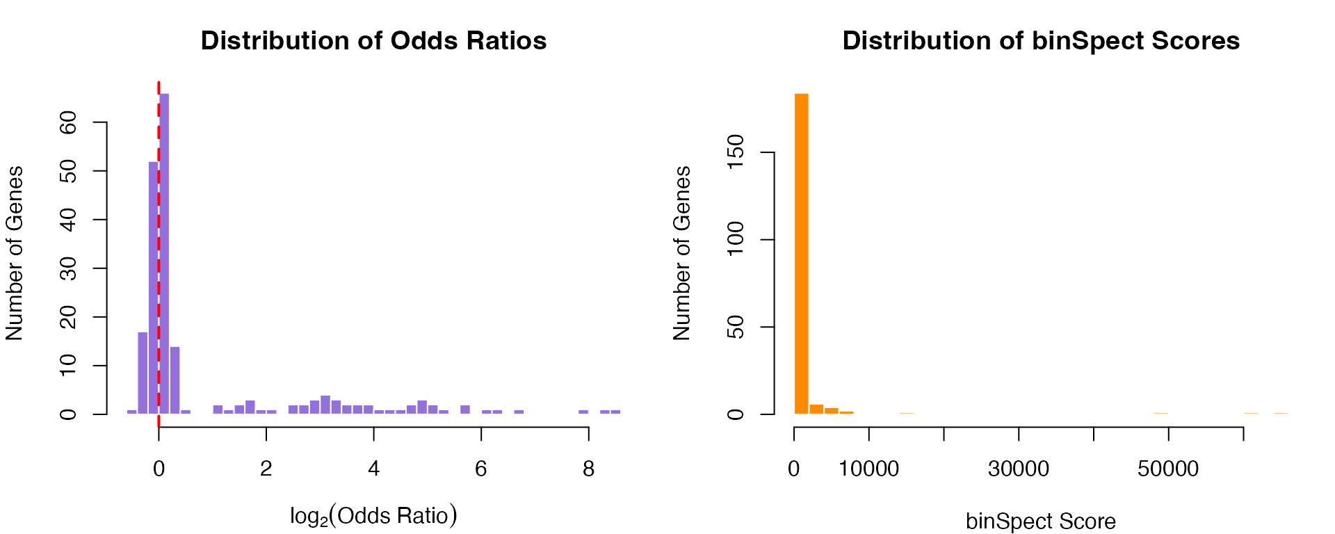

Method 3: SPARK-X (Kernel-Based Association)

Algorithm Overview

SPARK-X uses multiple spatial kernels to detect diverse pattern types, combining results via ACAT.

Kernels Used:

• 1 linear (projection) kernel
• 5 Gaussian RBF kernels (varying bandwidths)
• 5 cosine/periodic kernels (varying frequencies)

Running SPARK-X

# Run SPARK-X with mixture of kernels
# Note: Uses raw counts (not log-transformed)
results_sparkx <- CalSVG_SPARKX(
  expr_matrix = expr_counts,    # Raw counts recommended
  spatial_coords = coords,
  kernel_option = "mixture",    # All 11 kernels
  adjust_method = "BY",         # Benjamini-Yekutieli (conservative)
  verbose = FALSE
)

# Display top SVGs
cat("Top 10 SVGs by SPARK-X:\n")
#> Top 10 SVGs by SPARK-X:
head(results_sparkx[, c("gene", "p.value", "p.adj")], 10)
#>       gene       p.value         p.adj
#> 1   gene_4 8.282182e-179 9.736585e-176
#> 2  gene_10 9.435583e-163 5.546265e-160
#> 3  gene_14 6.294663e-160 2.466681e-157
#> 4  gene_12 2.134502e-158 6.273335e-156
#> 5   gene_5 2.592901e-154 6.096461e-152
#> 6  gene_18 7.617152e-144 1.492462e-141
#> 7  gene_15 2.459916e-134 4.131274e-132
#> 8  gene_25 3.889349e-134 5.715428e-132
#> 9  gene_22 5.640595e-134 7.367910e-132
#> 10 gene_17 3.852617e-130 4.529160e-128

Visualizing SPARK-X Results

par(mfrow = c(1, 2), mar = c(4, 4, 3, 1))

# Combined p-value distribution
hist(-log10(results_sparkx$p.value + 1e-300), breaks = 40,
     col = "seagreen", border = "white",
     xlab = expression(-log[10](p-value)),
     ylab = "Number of Genes",
     main = "SPARK-X P-value Distribution")

# Volcano-style plot
pval_log <- -log10(results_sparkx$p.adj + 1e-300)
plot(seq_along(pval_log), pval_log,
     pch = 19, cex = 0.6,
     col = ifelse(pval_log > -log10(0.05), "red", "gray50"),
     xlab = "Gene Index",
     ylab = expression(-log[10](adjusted~p-value)),
     main = "SPARK-X Significance Plot")
abline(h = -log10(0.05), col = "red", lty = 2)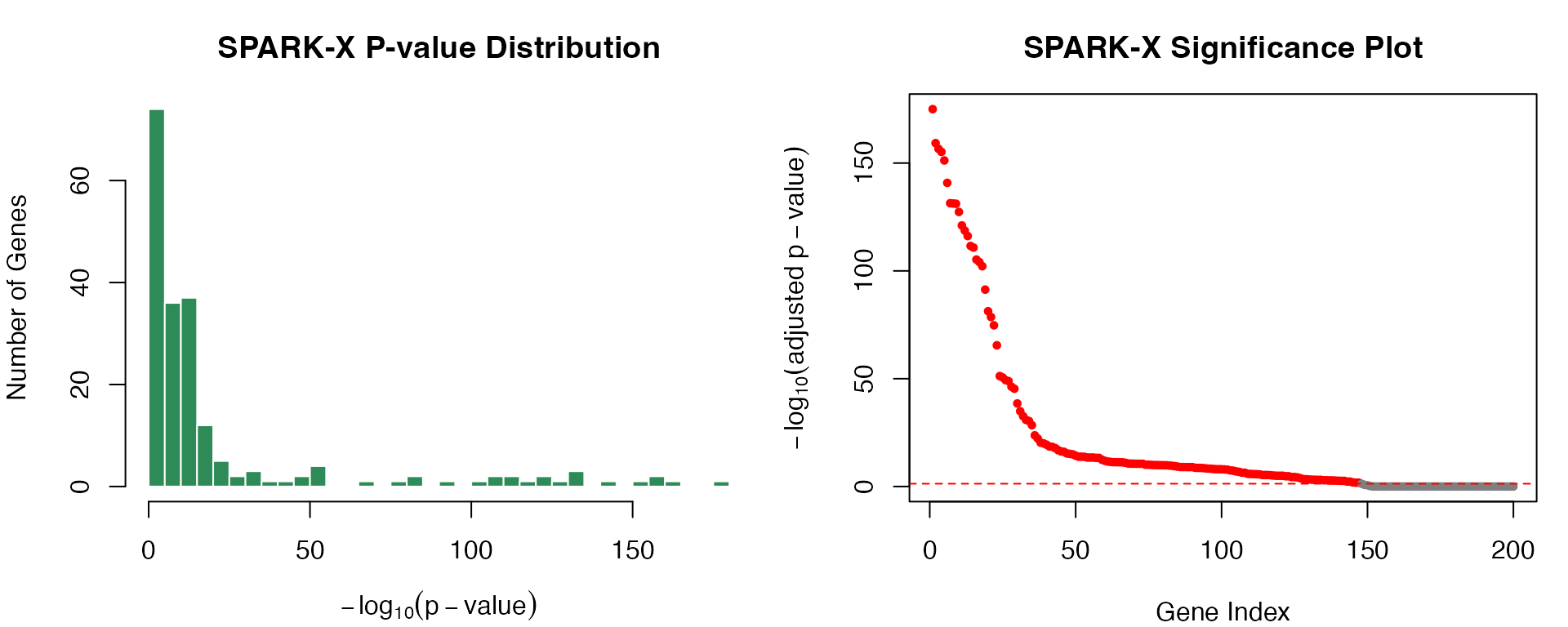

Method 4: Seurat (Moran’s I with Distance Weights)

Algorithm Overview

Seurat’s implementation uses inverse-squared distance weighting, emphasizing local spatial relationships.

$$w_{ij} = \frac{1}{d_{ij}^2}$$

Running Seurat Method

# Run Seurat Moran's I
results_seurat <- CalSVG_Seurat(
  expr_matrix = expr_log,
  spatial_coords = coords,
  weight_scheme = "inverse_squared",  # Seurat default
  adjust_method = "BH",
  verbose = FALSE
)

# Display top SVGs
cat("Top 10 SVGs by Seurat:\n")
#> Top 10 SVGs by Seurat:
head(results_seurat[, c("gene", "observed", "expected", "sd", "p.value", "p.adj")], 10)
#>       gene  observed     expected          sd p.value p.adj
#> 1   gene_7 0.6772728 -0.002004008 0.009605248       0     0
#> 2  gene_22 0.5457111 -0.002004008 0.009599242       0     0
#> 3  gene_17 0.5345832 -0.002004008 0.009597744       0     0
#> 4  gene_19 0.5149447 -0.002004008 0.009594016       0     0
#> 5   gene_9 0.5090348 -0.002004008 0.009574655       0     0
#> 6  gene_12 0.4738920 -0.002004008 0.009579223       0     0
#> 7  gene_25 0.4595807 -0.002004008 0.009597722       0     0
#> 8   gene_5 0.4564260 -0.002004008 0.009576880       0     0
#> 9  gene_14 0.4165174 -0.002004008 0.009595459       0     0
#> 10 gene_23 0.4098592 -0.002004008 0.009581536       0     0

Unified Interface: CalSVG()

For convenience, all methods can be accessed through a single unified interface:

# Example: Run MERINGUE through unified interface
results_unified <- CalSVG(
  expr_matrix = expr_log,
  spatial_coords = coords,
  method = "meringue",       # Options: meringue, binspect, sparkx, seurat, nnsvg, markvario
  network_method = "knn",
  k = 10,
  verbose = FALSE
)

cat("Unified interface results:\n")
#> Unified interface results:
head(results_unified[, c("gene", "p.value", "p.adj")], 5)
#>     gene p.value p.adj
#> 1 gene_1       0     0
#> 2 gene_2       0     0
#> 3 gene_3       0     0
#> 4 gene_4       0     0
#> 5 gene_5       0     0

---

Comprehensive Method Comparison

Performance Metrics

We evaluate all methods using standard classification metrics on the simulated data with known ground truth:

# Ground truth
truth <- gene_info$is_svg

# Function to calculate comprehensive metrics
calc_performance <- function(result, truth, pval_col = "p.adj", threshold = 0.05) {
  detected <- result[[pval_col]] < threshold
  detected[is.na(detected)] <- FALSE
  
  TP <- sum(truth & detected)
  FP <- sum(!truth & detected)
  FN <- sum(truth & !detected)
  TN <- sum(!truth & !detected)
  
  list(
    TP = TP, FP = FP, FN = FN, TN = TN,
    Sensitivity = TP / (TP + FN),
    Specificity = TN / (TN + FP),
    Precision = TP / max(TP + FP, 1),
    NPV = TN / max(TN + FN, 1),
    F1 = 2 * TP / max(2 * TP + FP + FN, 1),
    Accuracy = (TP + TN) / (TP + TN + FP + FN),
    MCC = (TP * TN - FP * FN) / sqrt((TP + FP) * (TP + FN) * (TN + FP) * (TN + FN) + 1e-10)
  )
}

# Calculate metrics for each method
metrics_list <- list(
  MERINGUE = calc_performance(results_meringue, truth),
  binSpect = calc_performance(results_binspect, truth),
  `SPARK-X` = calc_performance(results_sparkx, truth),
  Seurat = calc_performance(results_seurat, truth)
)

# Create metrics data frame
metrics_df <- do.call(rbind, lapply(names(metrics_list), function(m) {
  data.frame(
    Method = m,
    Sensitivity = metrics_list[[m]]$Sensitivity,
    Specificity = metrics_list[[m]]$Specificity,
    Precision = metrics_list[[m]]$Precision,
    F1 = metrics_list[[m]]$F1,
    MCC = metrics_list[[m]]$MCC
  )
}))

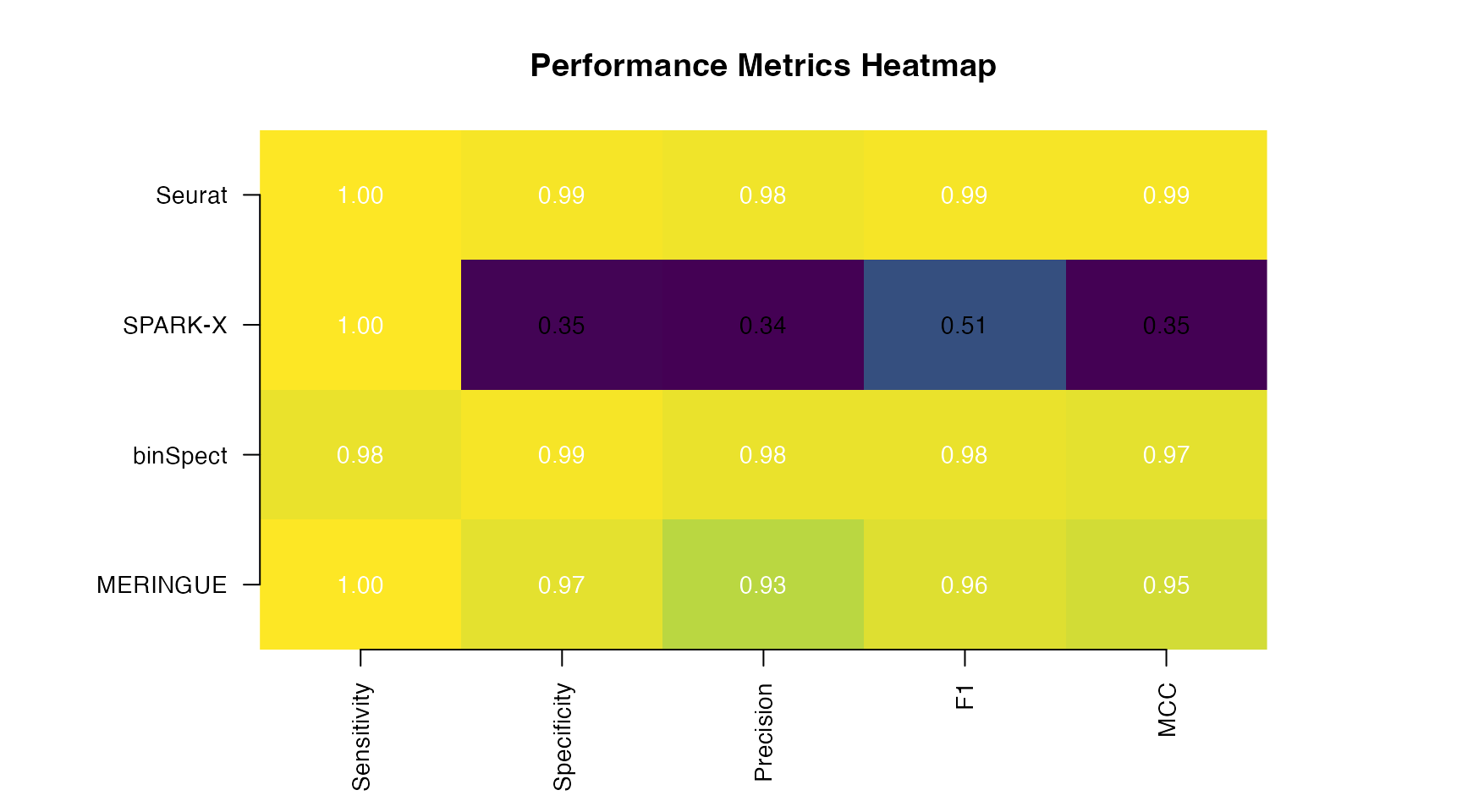
knitr::kable(metrics_df, digits = 3, 
             caption = "Performance Comparison on Simulated Data (FDR < 0.05)")

Performance Comparison on Simulated Data (FDR < 0.05)

Method	Sensitivity	Specificity	Precision	F1	MCC
MERINGUE	1.00	0.973	0.926	0.962	0.949
binSpect	0.98	0.993	0.980	0.980	0.973
SPARK-X	1.00	0.353	0.340	0.508	0.347
Seurat	1.00	0.993	0.980	0.990	0.987

Visual Performance Comparison

# Prepare data for heatmap
metrics_matrix <- as.matrix(metrics_df[, -1])
rownames(metrics_matrix) <- metrics_df$Method

# Create heatmap
par(mar = c(5, 8, 4, 6))
image(t(metrics_matrix), axes = FALSE,
      col = colorRampPalette(c("#440154", "#31688E", "#35B779", "#FDE725"))(100),
      main = "Performance Metrics Heatmap")

axis(1, at = seq(0, 1, length.out = ncol(metrics_matrix)),
     labels = colnames(metrics_matrix), las = 2, cex.axis = 0.9)
axis(2, at = seq(0, 1, length.out = nrow(metrics_matrix)),
     labels = rownames(metrics_matrix), las = 1, cex.axis = 0.9)

# Add values
for (i in 1:nrow(metrics_matrix)) {
  for (j in 1:ncol(metrics_matrix)) {
    text((j - 1) / (ncol(metrics_matrix) - 1),
         (i - 1) / (nrow(metrics_matrix) - 1),
         sprintf("%.2f", metrics_matrix[i, j]),
         cex = 0.9, col = ifelse(metrics_matrix[i, j] > 0.6, "white", "black"))
  }
}

ROC Curve Analysis

# Function to compute ROC curve
compute_roc <- function(scores, truth, higher_is_better = FALSE) {
  if (higher_is_better) {
    scores <- -scores
  }
  scores[is.na(scores)] <- max(scores, na.rm = TRUE) + 1
  
  thresholds <- sort(unique(c(-Inf, scores, Inf)))
  
  tpr <- fpr <- numeric(length(thresholds))
  for (i in seq_along(thresholds)) {
    predicted <- scores <= thresholds[i]
    tpr[i] <- sum(truth & predicted) / sum(truth)
    fpr[i] <- sum(!truth & predicted) / sum(!truth)
  }
  
  # Calculate AUC using trapezoidal rule
  ord <- order(fpr, tpr)
  fpr <- fpr[ord]
  tpr <- tpr[ord]
  auc <- sum(diff(fpr) * (head(tpr, -1) + tail(tpr, -1)) / 2)
  
  list(fpr = fpr, tpr = tpr, auc = auc)
}

# Compute ROC for each method
roc_meringue <- compute_roc(results_meringue$p.value, truth)
roc_binspect <- compute_roc(results_binspect$p.value, truth)
roc_sparkx <- compute_roc(results_sparkx$p.value, truth)
roc_seurat <- compute_roc(results_seurat$p.value, truth)

# Plot ROC curves
par(mar = c(5, 5, 4, 2))
plot(roc_meringue$fpr, roc_meringue$tpr, type = "l", lwd = 3, col = "#E41A1C",
     xlab = "False Positive Rate (1 - Specificity)",
     ylab = "True Positive Rate (Sensitivity)",
     main = "Receiver Operating Characteristic (ROC) Curves",
     xlim = c(0, 1), ylim = c(0, 1),
     cex.lab = 1.2, cex.main = 1.3)
lines(roc_binspect$fpr, roc_binspect$tpr, lwd = 3, col = "#377EB8")
lines(roc_sparkx$fpr, roc_sparkx$tpr, lwd = 3, col = "#4DAF4A")
lines(roc_seurat$fpr, roc_seurat$tpr, lwd = 3, col = "#984EA3")
abline(0, 1, lty = 2, col = "gray50", lwd = 2)

# Add AUC values to legend
legend("bottomright", 
       legend = c(
         sprintf("MERINGUE (AUC = %.3f)", roc_meringue$auc),
         sprintf("binSpect (AUC = %.3f)", roc_binspect$auc),
         sprintf("SPARK-X (AUC = %.3f)", roc_sparkx$auc),
         sprintf("Seurat (AUC = %.3f)", roc_seurat$auc)
       ),
       col = c("#E41A1C", "#377EB8", "#4DAF4A", "#984EA3"),
       lwd = 3, cex = 1.0, bty = "n")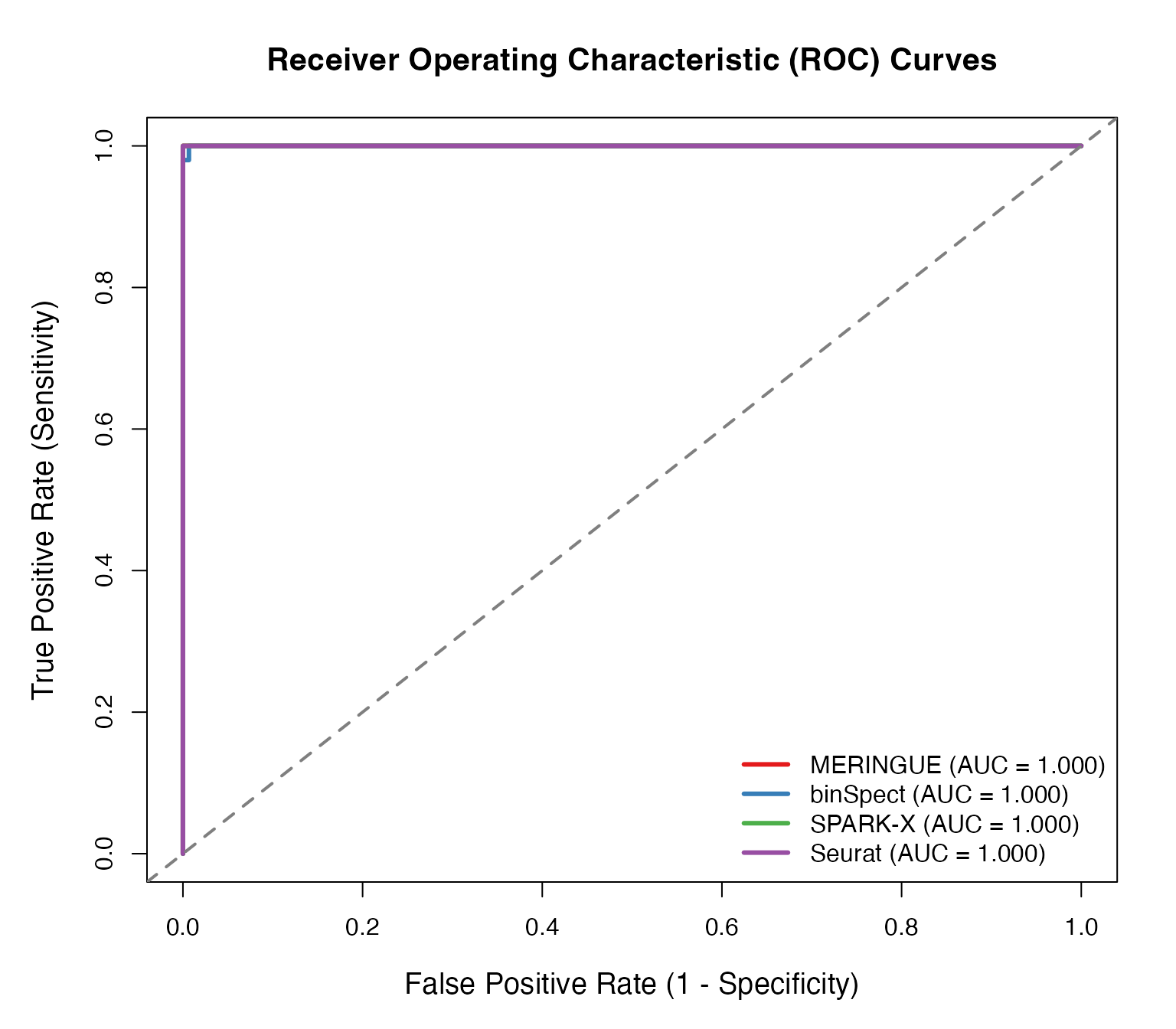

Overlap Analysis

# Get significant genes for each method
sig_genes <- list(
  MERINGUE = results_meringue$gene[results_meringue$p.adj < 0.05],
  binSpect = results_binspect$gene[results_binspect$p.adj < 0.05],
  SPARKX = results_sparkx$gene[results_sparkx$p.adj < 0.05],
  Seurat = results_seurat$gene[results_seurat$p.adj < 0.05]
)

# Calculate pairwise Jaccard indices
jaccard <- function(a, b) {
  length(intersect(a, b)) / length(union(a, b))
}

methods <- names(sig_genes)
jaccard_matrix <- matrix(0, length(methods), length(methods))
rownames(jaccard_matrix) <- colnames(jaccard_matrix) <- methods

for (i in seq_along(methods)) {
  for (j in seq_along(methods)) {
    jaccard_matrix[i, j] <- jaccard(sig_genes[[i]], sig_genes[[j]])
  }
}

# Visualize overlap
par(mfrow = c(1, 2), mar = c(5, 6, 4, 4))

# Jaccard similarity heatmap
image(jaccard_matrix, axes = FALSE,
      col = colorRampPalette(c("white", "steelblue", "darkblue"))(100),
      main = "Pairwise Jaccard Similarity")
axis(1, at = seq(0, 1, length.out = 4), labels = methods, las = 2, cex.axis = 0.9)
axis(2, at = seq(0, 1, length.out = 4), labels = methods, las = 1, cex.axis = 0.9)

for (i in 1:4) {
  for (j in 1:4) {
    text((j - 1) / 3, (i - 1) / 3, 
         sprintf("%.2f", jaccard_matrix[i, j]),
         cex = 1.0, col = ifelse(jaccard_matrix[i, j] > 0.5, "white", "black"))
  }
}

# Number of significant genes
barplot(sapply(sig_genes, length),
        col = c("#E41A1C", "#377EB8", "#4DAF4A", "#984EA3"),
        ylab = "Number of Significant Genes",
        main = "Number of SVGs Detected",
        las = 1, border = NA)
abline(h = sum(truth), lty = 2, col = "red", lwd = 2)
legend("topright", legend = "True SVGs (n=50)", lty = 2, col = "red", lwd = 2, bty = "n")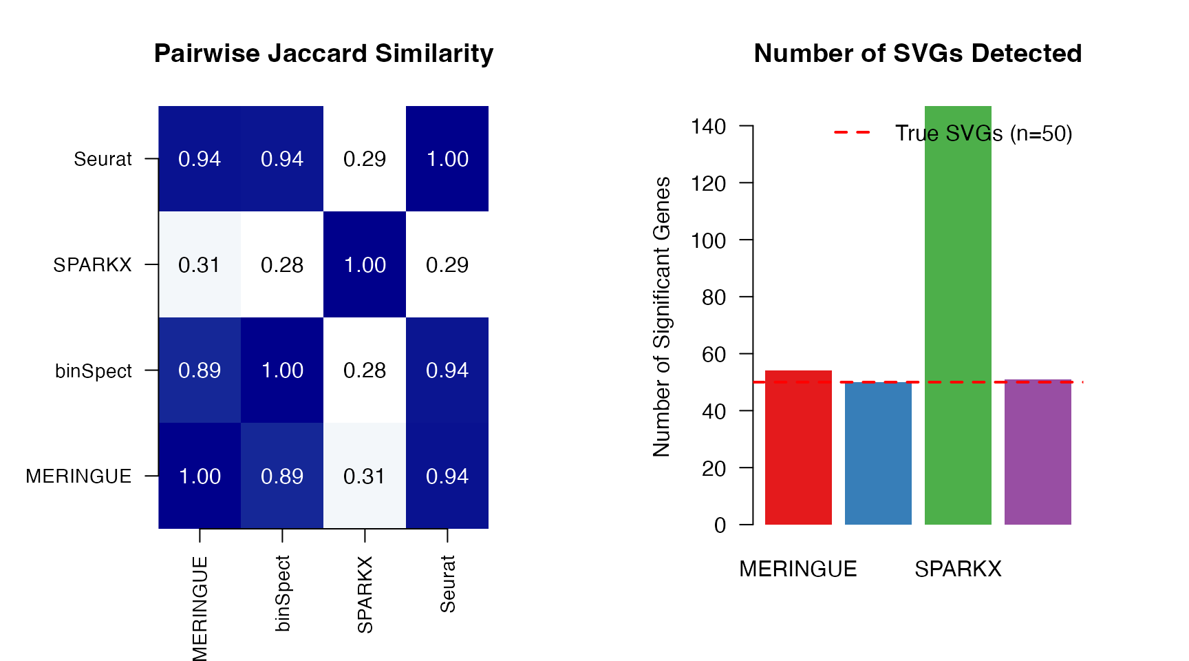

---

Advanced Analysis

Data Simulation for Custom Benchmarking

Generate custom simulated datasets with controlled parameters:

# Set seed for reproducibility
set.seed(2024)

# Generate custom dataset with specific parameters
sim_data <- simulate_spatial_data(
  n_spots = 400,              # Number of spatial locations
  n_genes = 150,              # Total genes
  n_svg = 30,                 # Number of true SVGs
  grid_type = "hexagonal",    # Spatial arrangement
  pattern_types = c("gradient", "hotspot", "periodic"),  # Pattern types to include
  mean_counts = 150,          # Mean expression level
  dispersion = 2.5            # Negative binomial dispersion
)

cat("Custom Simulation Summary:\n")
#> Custom Simulation Summary:
cat("  Spots:", ncol(sim_data$counts), "\n")
#>   Spots: 400
cat("  Genes:", nrow(sim_data$counts), "\n")
#>   Genes: 150
cat("  True SVGs:", sum(sim_data$gene_info$is_svg), "\n")
#>   True SVGs: 30
cat("\nPattern distribution:\n")
#> 
#> Pattern distribution:
print(table(sim_data$gene_info$pattern_type))
#> 
#> gradient  hotspot     none periodic 
#>       10       10      120       10

Parallelization for Large Datasets

# Demonstrate parallel processing
# Note: mclapply doesn't work on Windows; falls back to sequential

n_cores <- 2  # Adjust based on your system

t_start <- Sys.time()
results_parallel <- CalSVG_MERINGUE(
  expr_matrix = expr_log,
  spatial_coords = coords,
  n_threads = n_cores,
  verbose = FALSE
)
t_end <- Sys.time()

cat(sprintf("Parallel execution with %d cores: %.2f seconds\n", 
            n_cores, as.numeric(t_end - t_start, units = "secs")))
#> Parallel execution with 2 cores: 0.03 seconds

Gene Filtering Strategies

# Pre-filter genes to improve signal-to-noise and reduce computation

# Strategy 1: Expression threshold
gene_means <- rowMeans(expr_log)
expr_high <- expr_log[gene_means > quantile(gene_means, 0.1), ]
cat("After expression filter:", nrow(expr_high), "genes\n")
#> After expression filter: 180 genes

# Strategy 2: Variance filter
gene_vars <- apply(expr_high, 1, var)
expr_filtered <- expr_high[gene_vars > quantile(gene_vars, 0.25), ]
cat("After variance filter:", nrow(expr_filtered), "genes\n")
#> After variance filter: 135 genes

# Strategy 3: Coefficient of variation
cv <- apply(expr_high, 1, sd) / (rowMeans(expr_high) + 0.1)
expr_cv <- expr_high[cv > quantile(cv, 0.25), ]
cat("After CV filter:", nrow(expr_cv), "genes\n")
#> After CV filter: 135 genes

---

Practical Guidelines

Method Selection Framework

Scenario	Recommended Method	Rationale
Exploratory analysis	binSpect or Seurat	Fast, good general performance
Manuscript/publication	Multiple methods + consensus	Robust, reproducible
Large datasets (>10k spots)	SPARK-X	Scalable, efficient
Effect size needed	nnSVG	Provides prop_sv metric
Multiple pattern types expected	SPARK-X	Multi-kernel detection
Seurat workflow integration	CalSVG_Seurat	Compatible output format

Parameter Tuning Guidelines

Network Construction

Parameter	Default	When to Adjust
k (KNN neighbors)	10	Increase for sparse data, decrease for dense
network_method	“knn”	Use “delaunay” for uniform grids
filter_dist	NA	Set for large spatial extent

Statistical Testing

Parameter	Default	When to Adjust
adjust_method	“BH”	Use “BY” for conservative control
alternative	“greater”	Use “two.sided” for dispersed patterns

Computational Considerations

Method	Time Complexity	Memory	Parallelizable
MERINGUE	O(n·k·g)	Low	Yes
binSpect	O(n·g)	Low	Yes
SPARK-X	O(n²·g)	High	Yes
Seurat	O(n²·g)	High	Yes
nnSVG	O(n·m²·g)	Medium	Yes

---

Conclusion

The SVG package provides a comprehensive toolkit for spatially variable gene detection in spatial transcriptomics data. Key features include:

1. Unified Interface: Single function (CalSVG()) to access all methods
2. Rigorous Statistics: Proper null hypothesis testing and multiple testing correction
3. Scalability: C++ acceleration and parallelization support
4. Flexibility: Extensive parameter customization for diverse experimental designs
5. Reproducibility: Consistent output format across all methods

For questions, bug reports, or feature requests, please visit: https://github.com/Zaoqu-Liu/SVG

---

Session Information

sessionInfo()
#> R version 4.4.0 (2024-04-24)
#> Platform: aarch64-apple-darwin20
#> Running under: macOS 15.6.1
#> 
#> Matrix products: default
#> BLAS:   /Library/Frameworks/R.framework/Versions/4.4-arm64/Resources/lib/libRblas.0.dylib 
#> LAPACK: /Library/Frameworks/R.framework/Versions/4.4-arm64/Resources/lib/libRlapack.dylib;  LAPACK version 3.12.0
#> 
#> locale:
#> [1] C
#> 
#> time zone: Asia/Shanghai
#> tzcode source: internal
#> 
#> attached base packages:
#> [1] stats     graphics  grDevices utils     datasets  methods   base     
#> 
#> other attached packages:
#> [1] SVG_1.0.0
#> 
#> loaded via a namespace (and not attached):
#>  [1] cli_3.6.5           knitr_1.51          rlang_1.1.7        
#>  [4] xfun_0.56           otel_0.2.0          geometry_0.5.2     
#>  [7] textshaping_1.0.4   jsonlite_2.0.0      htmltools_0.5.9    
#> [10] CompQuadForm_1.4.4  ragg_1.5.0          sass_0.4.10        
#> [13] rmarkdown_2.30      abind_1.4-8         evaluate_1.0.5     
#> [16] jquerylib_0.1.4     MASS_7.3-65         fastmap_1.2.0      
#> [19] yaml_2.3.12         lifecycle_1.0.5     magic_1.6-1        
#> [22] compiler_4.4.0      codetools_0.2-20    fs_1.6.6           
#> [25] htmlwidgets_1.6.4   Rcpp_1.1.1          BiocParallel_1.40.2
#> [28] systemfonts_1.3.1   digest_0.6.39       R6_2.6.1           
#> [31] RANN_2.6.2          parallel_4.4.0      bslib_0.9.0        
#> [34] tools_4.4.0         pkgdown_2.1.3       cachem_1.1.0       
#> [37] desc_1.4.3

---

References