Introduction
SecAct (Secreted protein Activity inference) is an R package for inferring intercellular signaling activity mediated by secreted proteins. This quick start guide will help you get up and running in minutes.
Basic Usage
1. Load Example Data
SecAct includes example data from a clinical cohort study:
# Load expression matrix
data_path <- system.file("extdata/GSE100093.IFNG.expr.gz", package = "SecAct")
expr <- read.table(gzfile(data_path), sep = "\t", header = TRUE, row.names = 1)

cat("Expression matrix dimensions:", dim(expr)[1], "genes x", dim(expr)[2], "samples\n")
#> Expression matrix dimensions: 20174 genes x 17 samples
2. Infer Secreted Protein Activity
# Run activity inference (~30 seconds with nrand=100)
result <- SecAct.activity.inference(
  inputProfile = expr[, 1:5],  # Use first 5 samples for demo
  lambda = 5e5,
  nrand = 100
)

# View result structure
cat("\nResult contains:\n")
#>
#> Result contains:
cat("  beta (coefficients):", dim(result$beta), "\n")
#>   beta (coefficients): 1170 5
cat("  se (standard errors):", dim(result$se), "\n")
#>   se (standard errors): 1170 5
cat("  zscore:", dim(result$zscore), "\n")
#>   zscore: 1170 5
cat("  pvalue:", dim(result$pvalue), "\n")
#> pvalue: 1170 5Visualization
Activity Heatmap
# Select top variable secreted proteins
var_sp <- apply(result$zscore, 1, var)
top_var <- names(sort(var_sp, decreasing = TRUE))[1:15]

# Create heatmap
SecAct.heatmap.plot(result$zscore[top_var, ],
                    title = "Top Variable Secreted Proteins")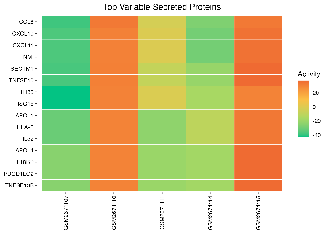
Secreted protein activity heatmap
Bar Plot
# Get activities for sample 1
activities <- result$zscore[, 1]

# Select top up and down regulated
n <- 8
top_up <- names(sort(activities, decreasing = TRUE))[1:n]
top_down <- names(sort(activities))[1:n]
selected <- c(top_up, top_down)

# Create bar plot
SecAct.bar.plot(activities[selected], title = "Sample 1 Activity")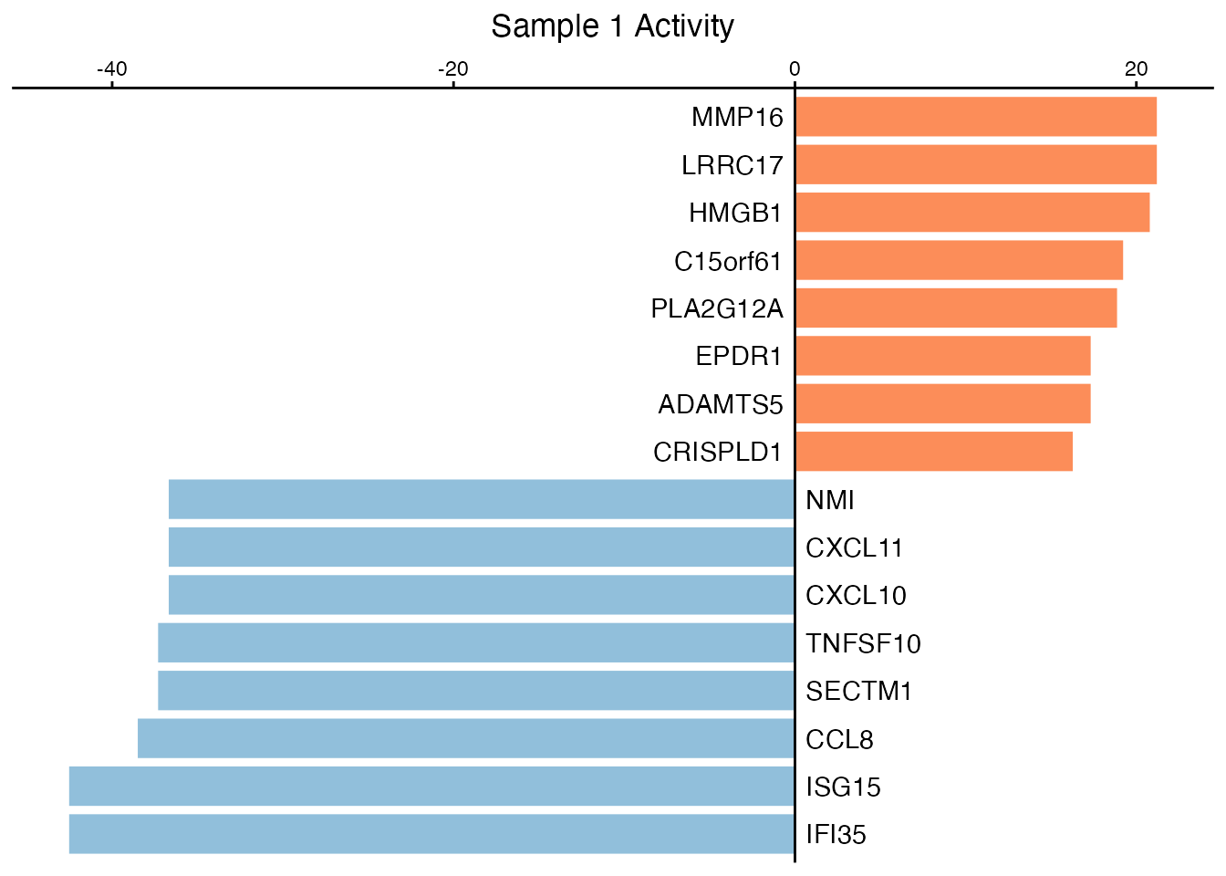
Top secreted proteins by activity
Lollipop Plot
SecAct.lollipop.plot(activities[selected], title = "Sample 1 Activity")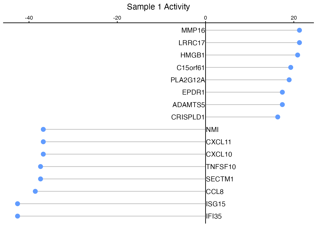
Lollipop visualization
Compare Treatment vs Control
A common use case is comparing two conditions:
# Load metadata
meta_path <- system.file("extdata/GSE100093.IFNG.meta", package = "SecAct")
meta <- read.table(meta_path, sep = "\t", header = TRUE, row.names = 1)

# Split by treatment
expr_treatment <- expr[, meta$Treatment == "Anti-IFNG"]
expr_control <- expr[, meta$Treatment == "Control"]

cat("Treatment samples:", ncol(expr_treatment), "\n")
#> Treatment samples: 8
cat("Control samples:", ncol(expr_control), "\n")
#> Control samples: 9
# Infer differential activity
diff_result <- SecAct.activity.inference(
  inputProfile = expr_treatment,
  inputProfile_control = expr_control,
  is.singleSampleLevel = FALSE,
  nrand = 100
)

# View IFNG activity change (should be negative due to anti-IFNG treatment)
cat("\nIFNG activity change:", round(diff_result$zscore["IFNG", "Change"], 2), "\n")
#>
#> IFNG activity change: -42.59
cat("(Negative = reduced activity in treatment group)\n")
#> (Negative = reduced activity in treatment group)
R vs GSL Implementation
SecAct provides two implementations:
# Pure R implementation (works everywhere)
set.seed(123)
r_result <- SecAct.inference.r(expr[, 1:3], nrand = 50)

# GSL implementation (faster, requires GSL)
set.seed(123)
gsl_result <- SecAct.inference.gsl(expr[, 1:3], nrand = 50)

# They produce highly correlated results
cat("Beta correlation:", round(cor(as.vector(r_result$beta),
                                    as.vector(gsl_result$beta)), 4), "\n")
#> Beta correlation: 0.9854
Workflow Summary
┌─────────────────────────────────────────────────────────────┐
│                    SecAct Workflow                          │
├─────────────────────────────────────────────────────────────┤
│                                                             │
│  1. Load Data ──────────────────────────────────────────►  │
│     (Expression matrix: genes × samples)                    │
│                                                             │
│  2. Activity Inference ─────────────────────────────────►  │
│     SecAct.activity.inference()                             │
│     SecAct.inference.r() or SecAct.inference.gsl()          │
│                                                             │
│  3. Visualization ──────────────────────────────────────►  │
│     SecAct.heatmap.plot()                                   │
│     SecAct.bar.plot()                                       │
│     SecAct.lollipop.plot()                                  │
│                                                             │
│  4. Downstream Analysis ────────────────────────────────►  │
│     SecAct.coxph.regression() (survival)                    │
│     SecAct.CCC.scRNAseq() (cell-cell communication)         │
│                                                             │
└─────────────────────────────────────────────────────────────┘
Next Steps
Explore more advanced tutorials:
-
Spatial Transcriptomics:
vignette("stPattern"),vignette("stCCC") -
Single-cell RNA-seq:
vignette("scCCC"),vignette("scState") -
Bulk RNA-seq:
vignette("bulkChange"),vignette("bulkCohort") -
Algorithm Details:
vignette("algorithm")
Getting Help
-
Documentation:
?SecAct.activity.inference - GitHub Issues: https://github.com/Zaoqu-Liu/SecAct/issues
- Contact: liuzaoqu@163.com
Session Info
sessionInfo()
#> R version 4.4.0 (2024-04-24)
#> Platform: aarch64-apple-darwin20
#> Running under: macOS 15.6.1
#>
#> Matrix products: default
#> BLAS:   /Library/Frameworks/R.framework/Versions/4.4-arm64/Resources/lib/libRblas.0.dylib
#> LAPACK: /Library/Frameworks/R.framework/Versions/4.4-arm64/Resources/lib/libRlapack.dylib;  LAPACK version 3.12.0
#>
#> locale:
#> [1] C
#>
#> time zone: Asia/Shanghai
#> tzcode source: internal
#>
#> attached base packages:
#> [1] stats     graphics  grDevices utils     datasets  methods   base
#>
#> other attached packages:
#> [1] SecAct_1.0.1
#>
#> loaded via a namespace (and not attached):
#>  [1] gtable_0.3.6       jsonlite_2.0.0     dplyr_1.1.4        compiler_4.4.0
#>  [5] tidyselect_1.2.1   Rcpp_1.1.1         stringr_1.6.0      dichromat_2.0-0.1
#>  [9] jquerylib_0.1.4    systemfonts_1.3.1  scales_1.4.0       textshaping_1.0.4
#> [13] yaml_2.3.12        fastmap_1.2.0      ggplot2_4.0.1      R6_2.6.1
#> [17] plyr_1.8.9         labeling_0.4.3     generics_0.1.4     knitr_1.51
#> [21] htmlwidgets_1.6.4  tibble_3.3.1       desc_1.4.3         pillar_1.11.1
#> [25] bslib_0.9.0        RColorBrewer_1.1-3 rlang_1.1.7        cachem_1.1.0
#> [29] stringi_1.8.7      xfun_0.56          fs_1.6.6           sass_0.4.10
#> [33] S7_0.2.1           otel_0.2.0         cli_3.6.5          withr_3.0.2
#> [37] pkgdown_2.1.3      magrittr_2.0.4     digest_0.6.39      grid_4.4.0
#> [41] lifecycle_1.0.5    vctrs_0.7.0        evaluate_1.0.5     glue_1.8.0
#> [45] farver_2.1.2       ragg_1.5.0         reshape2_1.4.5     rmarkdown_2.30
#> [49] pkgconfig_2.0.3    tools_4.4.0        htmltools_0.5.9