SpaTalk Visualization Guide
Zaoqu Liu
Maintainerliuzaoqu@163.com
2026-01-23
Source:vignettes/visualization.Rmd
visualization.RmdIntroduction
SpaTalk provides a comprehensive suite of visualization functions for exploring spatial transcriptomics data and cell-cell communication results. This vignette demonstrates the key plotting functions with real examples.
Setup
library(SpaTalk)
library(ggplot2)

# Load demo data
load(system.file("extdata", "starmap_data.rda", package = "SpaTalk"))
load(system.file("extdata", "starmap_meta.rda", package = "SpaTalk"))
data(lrpairs)
data(pathways)

# Create SpaTalk object
st_meta <- data.frame(
  cell = starmap_meta$cell,
  x = starmap_meta$x,
  y = starmap_meta$y
)

obj <- createSpaTalk(
  st_data = starmap_data,
  st_meta = st_meta,
  species = "Mouse",
  if_st_is_sc = TRUE,
  spot_max_cell = 1,
  celltype = starmap_meta$celltype
)

obj <- find_lr_path(obj, lrpairs, pathways, if_doParallel = FALSE)
#> Checking input data
#> Begin to filter lrpairs and pathways
#> ***Done***
#>

# Show available cell types
cat("Available cell types:", paste(unique(starmap_meta$celltype), collapse = ", "), "\n")
#> Available cell types: eL2_3, eL6, Astro, PVALB, Endo, VIP, SST, Smc, eL4, Micro, Oligo, eL5, Reln, HPC
Spatial Cell Type Visualization
plot_st_celltype_all
Display all cell types in a single spatial plot. This is one of the most commonly used visualizations.
plot_st_celltype_all(
  object = obj,
  size = 1.2
)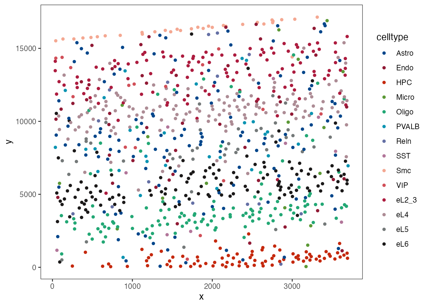
All cell types in spatial context
plot_st_celltype
Visualize specific cell type distributions in spatial coordinates.
plot_st_celltype(
  object = obj,
  celltype = "eL6",
  size = 1.5
)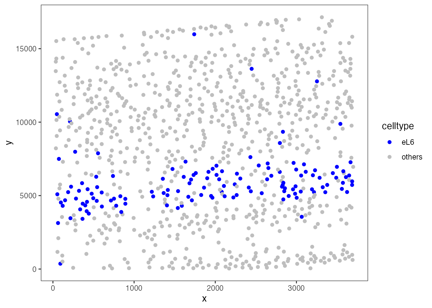
Spatial distribution of eL6 cells
plot_st_celltype_density
Kernel density estimation of cell type spatial distributions.
plot_st_celltype_density(
  object = obj,
  celltype = "eL6",
  type = "contour"
)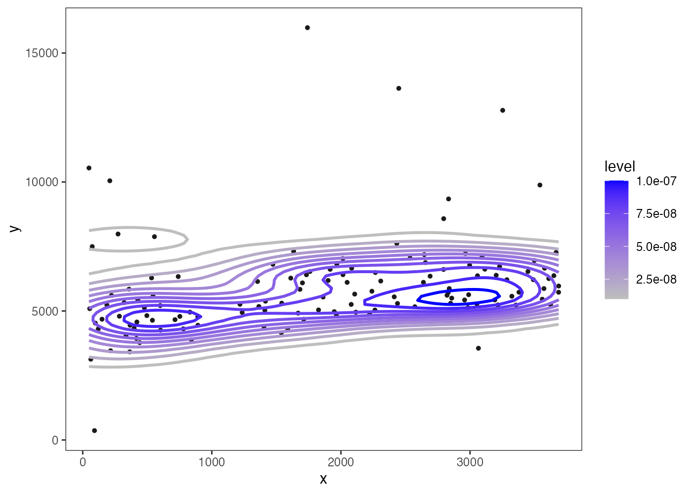
Cell type density map for eL6
Gene Expression Visualization
plot_st_gene
Visualize gene expression patterns in spatial coordinates.
# Get available genes
genes <- rownames(obj@data$rawdata)
cat("Total genes:", length(genes), "\n")
#> Total genes: 996

# Plot first available gene
plot_st_gene(
  object = obj,
  gene = genes[1],
  size = 1.5
)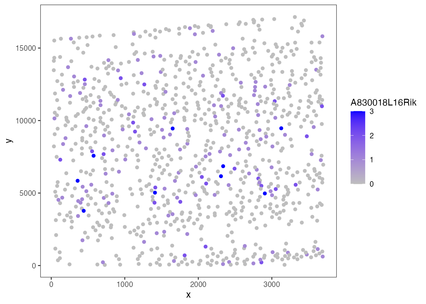
Spatial gene expression
Advanced Visualizations (After CCI Analysis)
The following visualizations require running dec_cci()
or dec_cci_all() first:
# Run CCI analysis for demonstration
obj <- dec_cci(
  object = obj,
  celltype_sender = "eL6",
  celltype_receiver = "PVALB",
  if_doParallel = FALSE
)
#> Begin to find LR pairs
#>

# Check results
if(nrow(obj@lrpair) > 0) {
  cat("Found", nrow(obj@lrpair), "significant LR pairs\n")
  print(head(obj@lrpair[, c("ligand", "receptor", "lr_co_ratio", "score")]))
}
#> Found 1 significant LR pairs
#>   ligand receptor lr_co_ratio     score
#> 5  Inhba   Acvr1c   0.1666667 0.8541642
plot_ccdist
Distribution of distances between interacting cell types.
plot_ccdist(
  object = obj,
  celltype_sender = "eL6",
  celltype_receiver = "PVALB"
)
Cell-cell distance distribution between eL6 and PVALB
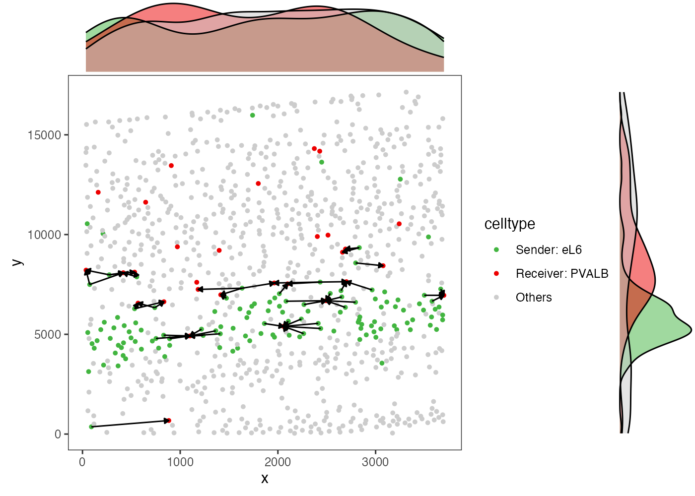
plot_lrpair
Spatial visualization of specific ligand-receptor pair interactions (if significant pairs found).
if(nrow(obj@lrpair) > 0) {
  lr <- obj@lrpair[1, ]
  plot_lrpair(
    object = obj,
    ligand = lr$ligand,
    receptor = lr$receptor,
    celltype_sender = "eL6",
    celltype_receiver = "PVALB",
    size = 1.2
  )
} else {
  cat("No significant LR pairs found for visualization\n")
}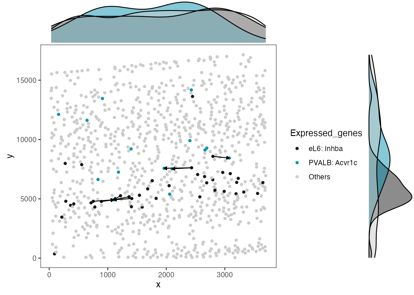
Spatial LR pair visualization
Customization Tips
Custom Themes
SpaTalk uses ggplot2 for all visualizations. You can easily customize:
p <- plot_st_celltype_all(obj, size = 1)

p +
  theme_minimal() +
  theme(
    legend.position = "bottom",
    plot.title = element_text(hjust = 0.5, size = 14, face = "bold")
  ) +
  labs(title = "STARmap Cell Type Distribution")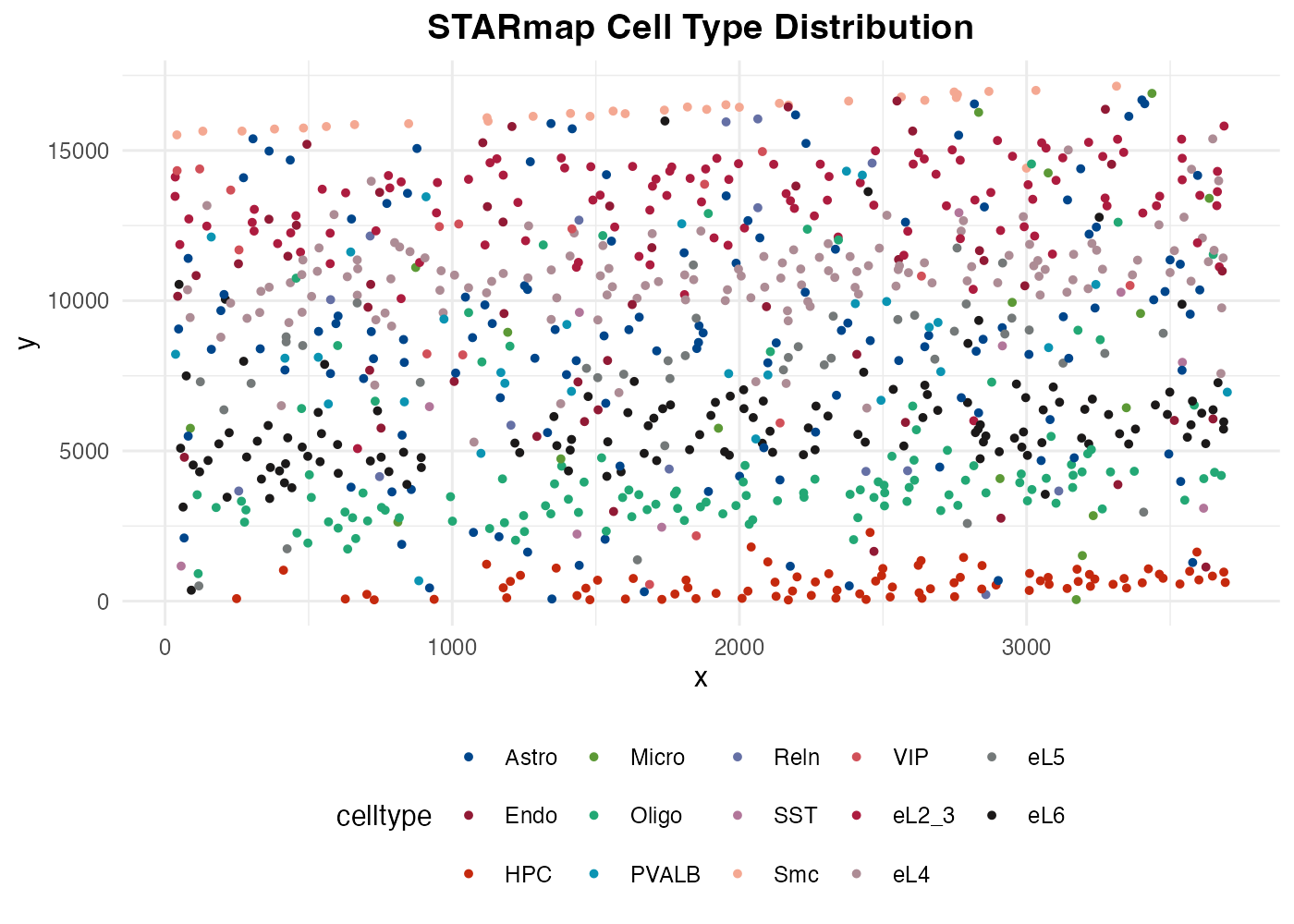
Customized plot with different theme
Summary of Visualization Functions
| Function | Description | Input Required |
|---|---|---|
plot_st_celltype |
Single cell type spatial | SpaTalk object |
plot_st_celltype_all |
All cell types spatial | SpaTalk object |
plot_st_celltype_percent |
Pie chart per spot | Deconvolved object |
plot_st_celltype_density |
Density heatmap | SpaTalk object |
plot_st_gene |
Gene expression spatial | SpaTalk object |
plot_st_pie |
Pie chart composition | Deconvolved object |
plot_cci_lrpairs |
CCI chord diagram | After dec_cci |
plot_lrpair |
LR pair spatial | After dec_cci |
plot_lrpair_vln |
LR violin plot | After dec_cci |
plot_lr_path |
LR-pathway network | After dec_cci |
plot_path2gene |
Pathway heatmap | After dec_cci |
plot_st_cor_heatmap |
Correlation heatmap | SpaTalk object |
plot_ccdist |
Distance distribution | SpaTalk object |
Session Info
sessionInfo()
#> R version 4.4.0 (2024-04-24)
#> Platform: aarch64-apple-darwin20
#> Running under: macOS 15.6.1
#>
#> Matrix products: default
#> BLAS:   /Library/Frameworks/R.framework/Versions/4.4-arm64/Resources/lib/libRblas.0.dylib
#> LAPACK: /Library/Frameworks/R.framework/Versions/4.4-arm64/Resources/lib/libRlapack.dylib;  LAPACK version 3.12.0
#>
#> locale:
#> [1] C
#>
#> time zone: Asia/Shanghai
#> tzcode source: internal
#>
#> attached base packages:
#> [1] parallel  stats     graphics  grDevices utils     datasets  methods
#> [8] base
#>
#> other attached packages:
#> [1] SpaTalk_2.0.0     doParallel_1.0.17 iterators_1.0.14  foreach_1.5.2
#> [5] ggalluvial_0.12.5 ggplot2_4.0.1
#>
#> loaded via a namespace (and not attached):
#>   [1] RColorBrewer_1.1-3     jsonlite_2.0.0         magrittr_2.0.4
#>   [4] spatstat.utils_3.2-1   farver_2.1.2           rmarkdown_2.30
#>   [7] fs_1.6.6               ragg_1.5.0             vctrs_0.7.0
#>  [10] ROCR_1.0-11            spatstat.explore_3.6-0 rstatix_0.7.3
#>  [13] htmltools_0.5.9        progress_1.2.3         broom_1.0.11
#>  [16] Formula_1.2-5          sass_0.4.10            sctransform_0.4.3
#>  [19] parallelly_1.46.1      KernSmooth_2.23-26     bslib_0.9.0
#>  [22] htmlwidgets_1.6.4      desc_1.4.3             ica_1.0-3
#>  [25] plyr_1.8.9             plotly_4.11.0          zoo_1.8-15
#>  [28] cachem_1.1.0           igraph_2.2.1           mime_0.13
#>  [31] lifecycle_1.0.5        pkgconfig_2.0.3        Matrix_1.7-4
#>  [34] R6_2.6.1               fastmap_1.2.0          fitdistrplus_1.2-4
#>  [37] future_1.69.0          shiny_1.12.1           digest_0.6.39
#>  [40] patchwork_1.3.2        Seurat_4.4.0           tensor_1.5.1
#>  [43] irlba_2.3.5.1          textshaping_1.0.4      ggpubr_0.6.2
#>  [46] labeling_0.4.3         progressr_0.18.0       spatstat.sparse_3.1-0
#>  [49] httr_1.4.7             polyclip_1.10-7        abind_1.4-8
#>  [52] compiler_4.4.0         withr_3.0.2            backports_1.5.0
#>  [55] S7_0.2.1               carData_3.0-5          ggforce_0.5.0
#>  [58] ggsignif_0.6.4         MASS_7.3-65            rappdirs_0.3.4
#>  [61] ggsci_4.2.0            tools_4.4.0            lmtest_0.9-40
#>  [64] otel_0.2.0             scatterpie_0.2.6       httpuv_1.6.16
#>  [67] future.apply_1.20.1    goftest_1.2-3          glue_1.8.0
#>  [70] nlme_3.1-168           promises_1.5.0         grid_4.4.0
#>  [73] Rtsne_0.17             cluster_2.1.8.1        reshape2_1.4.5
#>  [76] generics_0.1.4         isoband_0.3.0          gtable_0.3.6
#>  [79] spatstat.data_3.1-9    tzdb_0.5.0             tidyr_1.3.2
#>  [82] data.table_1.18.0      hms_1.1.4              car_3.1-3
#>  [85] sp_2.2-0               spatstat.geom_3.6-1    RcppAnnoy_0.0.23
#>  [88] ggrepel_0.9.6          RANN_2.6.2             pillar_1.11.1
#>  [91] stringr_1.6.0          yulab.utils_0.2.3      ggExtra_0.11.0
#>  [94] later_1.4.5            splines_4.4.0          tweenr_2.0.3
#>  [97] dplyr_1.1.4            lattice_0.22-7         survival_3.8-3
#> [100] deldir_2.0-4           tidyselect_1.2.1       miniUI_0.1.2
#> [103] pbapply_1.7-4          knitr_1.51             gridExtra_2.3
#> [106] scattermore_1.2        xfun_0.56              matrixStats_1.5.0
#> [109] pheatmap_1.0.13        stringi_1.8.7          ggfun_0.2.0
#> [112] lazyeval_0.2.2         yaml_2.3.12            evaluate_1.0.5
#> [115] codetools_0.2-20       tibble_3.3.1           cli_3.6.5
#> [118] uwot_0.2.4             xtable_1.8-4           reticulate_1.44.1
#> [121] systemfonts_1.3.1      jquerylib_0.1.4        dichromat_2.0-0.1
#> [124] Rcpp_1.1.1             globals_0.18.0         spatstat.random_3.4-3
#> [127] png_0.1-8              spatstat.univar_3.1-6  readr_2.1.6
#> [130] pkgdown_2.1.3          NNLM_0.4.4             prettyunits_1.2.0
#> [133] listenv_0.10.0         viridisLite_0.4.2      scales_1.4.0
#> [136] ggridges_0.5.7         SeuratObject_4.1.4     leiden_0.4.3.1
#> [139] purrr_1.2.1            crayon_1.5.3           rlang_1.1.7
#> [142] cowplot_1.2.0