Mathematical Foundation of NicheNet

Introduction

This vignette provides a rigorous mathematical treatment of the NicheNet algorithm. We describe the probabilistic framework underlying ligand-target predictions and the statistical methods used for ligand activity inference.

Network Representation

Graph Notation

Let $\mathcal{G} = (V, E, W)$ be a weighted directed graph where:

$V = \{v_1, v_2, \ldots, v_n\}$ is the set of genes/proteins
$E \subseteq V \times V$ is the set of directed edges
$W: E \to \mathbb{R}^+$ assigns positive weights to edges

The adjacency matrix $\mathbf{A} \in \mathbb{R}^{n \times n}$ is defined as:

$A_{ij} = \begin{cases} W(v_i, v_j) & \text{if } (v_i, v_j) \in E \\ 0 & \text{otherwise} \end{cases}$

Multi-Source Integration

Given $K$ data sources with edge sets $E_1, E_2, \ldots, E_K$ and source weights $\mathbf{w} = (w_1, \ldots, w_K)^T$ , the integrated adjacency matrix is:

$\mathbf{A}^{int} = \sum_{k=1}^{K} w_k \cdot \mathbf{A}^{(k)}$

where $\mathbf{A}^{(k)}$ is the binary adjacency matrix for source $k$ .

# Simulate multi-source integration
set.seed(42)
n_sources <- 5
source_names <- c("OmniPath", "KEGG", "Reactome", "TRRUST", "RegNetwork")
weights <- c(0.8, 0.6, 0.7, 0.5, 0.4)

# Create example edge contributions
edge_contributions <- data.frame(
  source = rep(source_names, each = 100),
  weight = rep(weights, each = 100),
  edge_present = rbinom(500, 1, rep(c(0.3, 0.5, 0.4, 0.6, 0.2), each = 100))
) %>%
  mutate(contribution = weight * edge_present)

# Summarize
source_summary <- edge_contributions %>%
  group_by(source) %>%
  summarise(
    coverage = mean(edge_present),
    avg_contribution = mean(contribution),
    weight = first(weight)
  ) %>%
  arrange(desc(avg_contribution))

ggplot(source_summary, aes(x = reorder(source, avg_contribution), y = coverage, fill = weight)) +
  geom_col() +
  geom_text(aes(label = sprintf("w=%.1f", weight)), hjust = -0.1, size = 3.5) +
  coord_flip() +
  scale_fill_gradient(low = "#cfe2ff", high = "#0d6efd") +
  labs(
    title = "Data Source Contributions",
    subtitle = "Edge coverage weighted by source reliability",
    x = "Data Source",
    y = "Edge Coverage",
    fill = "Weight"
  ) +
  theme_minimal() +
  theme(plot.title = element_text(face = "bold"))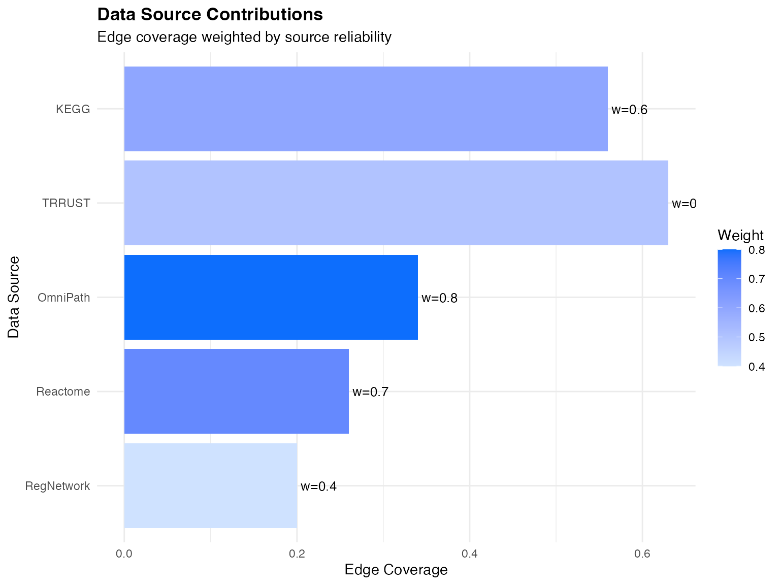

Visualization of multi-source network integration

Hub Correction

Motivation

Highly connected nodes (hubs) can dominate random walk-based methods. To mitigate this, we apply degree-based normalization.

Mathematical Formulation

Let $d_j^{in} = \sum_i A_{ij}$ be the in-degree of node $j$ . The hub-corrected weight matrix is:

$\tilde{A}_{ij} = A_{ij} \cdot (d_j^{in})^{-h}$

where $h \in [0, 1]$ is the hub correction parameter: - $h = 0$ : No correction - $h = 1$ : Full inverse-degree normalization

# Demonstrate hub correction effect
hub_demo <- data.frame(
  in_degree = 1:100,
  h_0 = 1,
  h_0.25 = (1:100)^(-0.25),
  h_0.5 = (1:100)^(-0.5),
  h_0.75 = (1:100)^(-0.75),
  h_1 = (1:100)^(-1)
) %>%
  pivot_longer(-in_degree, names_to = "h_value", values_to = "correction_factor") %>%
  mutate(h_value = factor(h_value, 
                          levels = c("h_0", "h_0.25", "h_0.5", "h_0.75", "h_1"),
                          labels = c("h=0", "h=0.25", "h=0.5", "h=0.75", "h=1")))

ggplot(hub_demo, aes(x = in_degree, y = correction_factor, color = h_value)) +
  geom_line(linewidth = 1) +
  scale_y_log10() +
  scale_color_viridis_d() +
  labs(
    title = "Hub Correction Factors",
    subtitle = expression(paste("Correction = ", d^{-h}, " for different h values")),
    x = "In-degree",
    y = "Correction Factor (log scale)",
    color = "Hub Parameter"
  ) +
  theme_minimal() +
  theme(
    plot.title = element_text(face = "bold"),
    legend.position = "right"
  )

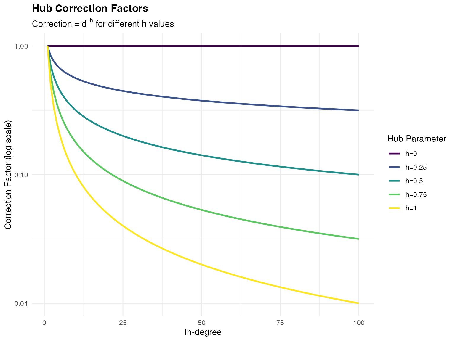
Effect of hub correction on edge weights

Personalized PageRank

Random Walk Interpretation

Consider a random walker on graph $\mathcal{G}$ :

Start at ligand node $L$
At each step:
- With probability $\alpha$ : follow an outgoing edge (weighted by $\tilde{A}$ )
- With probability $(1-\alpha)$ : restart at $L$

The stationary distribution $\boldsymbol{\pi}_L$ satisfies:

$\boldsymbol{\pi}_L = (1-\alpha) \mathbf{e}_L + \alpha \mathbf{P}^T \boldsymbol{\pi}_L$

where: - $\mathbf{e}_L$ is the indicator vector for ligand $L$ - $\mathbf{P} = \mathbf{D}^{-1}\tilde{\mathbf{A}}$ is the row-normalized transition matrix - $\mathbf{D} = \text{diag}(\sum_j \tilde{A}_{ij})$ is the out-degree matrix

Closed-Form Solution

Rearranging:

$\boldsymbol{\pi}_L = (1-\alpha)(\mathbf{I} - \alpha \mathbf{P}^T)^{-1} \mathbf{e}_L$

Iterative Computation

For large networks, we use power iteration:

$\boldsymbol{\pi}_L^{(t+1)} = (1-\alpha) \mathbf{e}_L + \alpha \mathbf{P}^T \boldsymbol{\pi}_L^{(t)}$

Convergence is guaranteed for $\alpha < 1$ .

# Simulate PPR convergence
set.seed(123)
n_nodes <- 50
alpha <- 0.5
max_iter <- 30

# Create random transition matrix
P <- matrix(runif(n_nodes^2), n_nodes, n_nodes)
P <- P / rowSums(P)

# Start vector (ligand at position 1)
e_L <- rep(0, n_nodes)
e_L[1] <- 1

# Iterate
pi_history <- matrix(NA, max_iter, n_nodes)
pi <- e_L

for (t in 1:max_iter) {
  pi <- (1-alpha) * e_L + alpha * t(P) %*% pi
  pi_history[t,] <- pi
}

# Plot convergence for top nodes
convergence_df <- data.frame(
  iteration = rep(1:max_iter, 5),
  node = rep(paste0("Node ", 1:5), each = max_iter),
  ppr = c(pi_history[,1], pi_history[,2], pi_history[,3], 
          pi_history[,4], pi_history[,5])
)

ggplot(convergence_df, aes(x = iteration, y = ppr, color = node)) +
  geom_line(linewidth = 1) +
  geom_point(size = 0.8) +
  scale_color_brewer(palette = "Set1") +
  labs(
    title = "PageRank Convergence",
    subtitle = paste("Damping factor α =", alpha),
    x = "Iteration",
    y = "PageRank Score",
    color = "Node"
  ) +
  theme_minimal() +
  theme(
    plot.title = element_text(face = "bold"),
    legend.position = "right"
  )

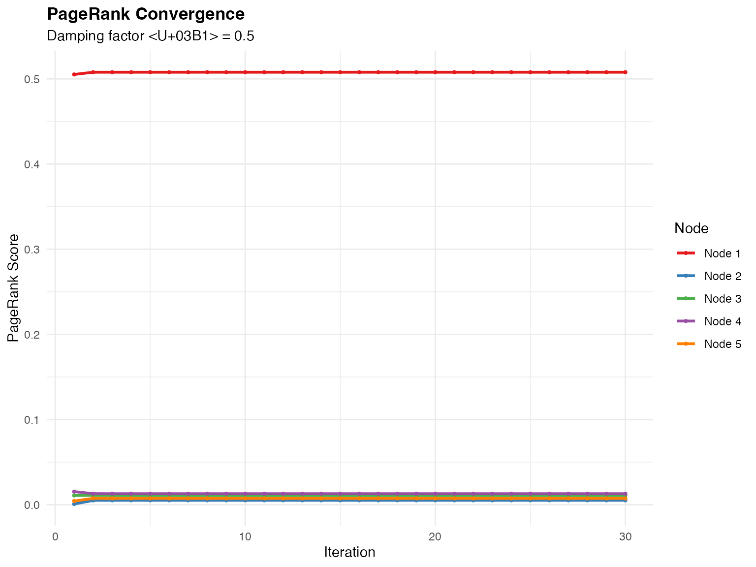
Personalized PageRank convergence

Ligand-Target Matrix Construction

Definition

The ligand-target matrix $\mathbf{M} \in \mathbb{R}^{|L| \times |G|}$ contains regulatory potential scores:

$M_{\ell g} = \boldsymbol{\pi}_\ell(g) \cdot R_g$

where: - $\boldsymbol{\pi}_\ell(g)$ is the PPR score from ligand $\ell$ to gene $g$ - $R_g$ is an optional regulatory weight (e.g., from GRN)

Sparsification

To improve computational efficiency and reduce noise:

$\tilde{M}_{\ell g} = \begin{cases} M_{\ell g} & \text{if } M_{\ell g} > Q_\tau(\mathbf{M}_\ell) \\ 0 & \text{otherwise} \end{cases}$

where $Q_\tau$ is the $\tau$ -quantile (default $\tau = 0.99$ ).

Ligand Activity Inference

Statistical Framework

Binary Classification Setup

For a ligand $\ell$ with scores $\mathbf{m}_\ell = (M_{\ell 1}, \ldots, M_{\ell G})$ and target indicator $\mathbf{y} \in \{0, 1\}^G$ :

Positive class: $\mathcal{P} = \{g : y_g = 1\}$ (genes of interest)
Negative class: $\mathcal{N} = \{g : y_g = 0\}$ (background genes)

AUROC Computation

$\text{AUROC} = \frac{\sum_{i \in \mathcal{P}} \sum_{j \in \mathcal{N}} \mathbf{1}[m_i > m_j]}{|\mathcal{P}| \cdot |\mathcal{N}|}$

Interpretation: Probability that a randomly chosen positive has higher score than a randomly chosen negative.

# Generate example ROC curve
set.seed(456)
n_pos <- 50
n_neg <- 200

# Good classifier
scores_pos <- rnorm(n_pos, mean = 0.7, sd = 0.2)
scores_neg <- rnorm(n_neg, mean = 0.3, sd = 0.2)

all_scores <- c(scores_pos, scores_neg)
all_labels <- c(rep(1, n_pos), rep(0, n_neg))

# Compute ROC
thresholds <- sort(unique(all_scores), decreasing = TRUE)
tpr <- sapply(thresholds, function(t) sum(scores_pos >= t) / n_pos)
fpr <- sapply(thresholds, function(t) sum(scores_neg >= t) / n_neg)

roc_df <- data.frame(fpr = c(0, fpr, 1), tpr = c(0, tpr, 1))

# Calculate AUROC
auroc <- sum(diff(c(0, fpr, 1)) * (c(0, tpr, 1)[-1] + c(0, tpr, 1)[-length(c(0,tpr,1))]) / 2)

ggplot(roc_df, aes(x = fpr, y = tpr)) +
  geom_line(color = "#0d6efd", linewidth = 1.2) +
  geom_abline(slope = 1, intercept = 0, linetype = "dashed", color = "gray50") +
  geom_ribbon(aes(ymin = fpr, ymax = tpr), fill = "#0d6efd", alpha = 0.2) +
  annotate("text", x = 0.6, y = 0.3, 
           label = sprintf("AUROC = %.3f", auroc), 
           size = 5, fontface = "bold") +
  labs(
    title = "Receiver Operating Characteristic (ROC) Curve",
    x = "False Positive Rate (1 - Specificity)",
    y = "True Positive Rate (Sensitivity)"
  ) +
  theme_minimal() +
  theme(plot.title = element_text(face = "bold")) +
  coord_equal()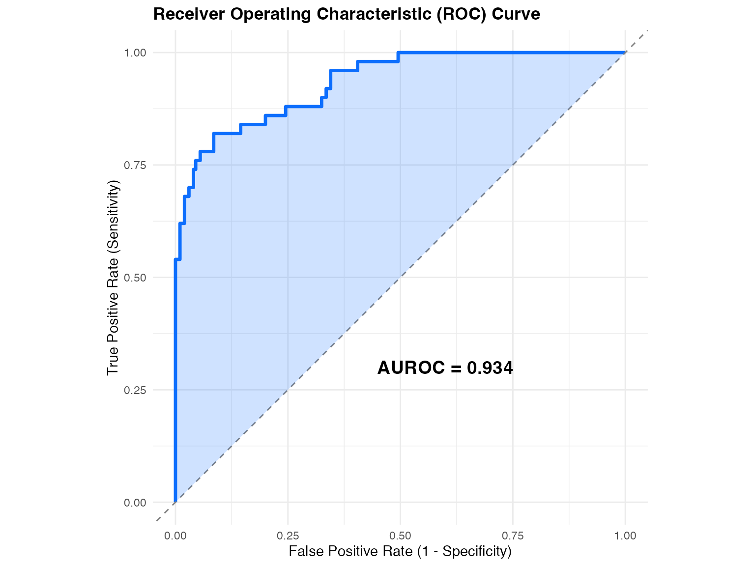

AUROC computation illustrated

AUPR Computation

$\text{AUPR} = \sum_{k=1}^{n} (R_k - R_{k-1}) \cdot P_k$

where at threshold $k$ : - $P_k = \frac{TP_k}{TP_k + FP_k}$ (Precision) - $R_k = \frac{TP_k}{|\mathcal{P}|}$ (Recall)

Baseline Correction

Random classifier AUPR equals the class prior:

$\text{AUPR}_{random} = \frac{|\mathcal{P}|}{|\mathcal{P}| + |\mathcal{N}|}$

Corrected AUPR:

$\text{AUPR}_{corrected} = \text{AUPR} - \text{AUPR}_{random}$

# Compute PR curve
precision <- sapply(thresholds, function(t) {
  tp <- sum(scores_pos >= t)
  fp <- sum(scores_neg >= t)
  if (tp + fp == 0) return(1)
  tp / (tp + fp)
})
recall <- sapply(thresholds, function(t) sum(scores_pos >= t) / n_pos)

pr_df <- data.frame(recall = c(0, recall), precision = c(1, precision))
baseline <- n_pos / (n_pos + n_neg)

# Calculate AUPR
aupr <- sum(diff(c(0, recall)) * precision)

ggplot(pr_df, aes(x = recall, y = precision)) +
  geom_line(color = "#198754", linewidth = 1.2) +
  geom_hline(yintercept = baseline, linetype = "dashed", color = "gray50") +
  geom_ribbon(aes(ymin = baseline, ymax = precision), fill = "#198754", alpha = 0.2) +
  annotate("text", x = 0.7, y = baseline + 0.05, 
           label = sprintf("Baseline = %.3f", baseline), color = "gray40") +
  annotate("text", x = 0.3, y = 0.9, 
           label = sprintf("AUPR = %.3f\nCorrected = %.3f", aupr, aupr - baseline), 
           size = 4, fontface = "bold") +
  labs(
    title = "Precision-Recall Curve",
    x = "Recall (Sensitivity)",
    y = "Precision (PPV)"
  ) +
  theme_minimal() +
  theme(plot.title = element_text(face = "bold"))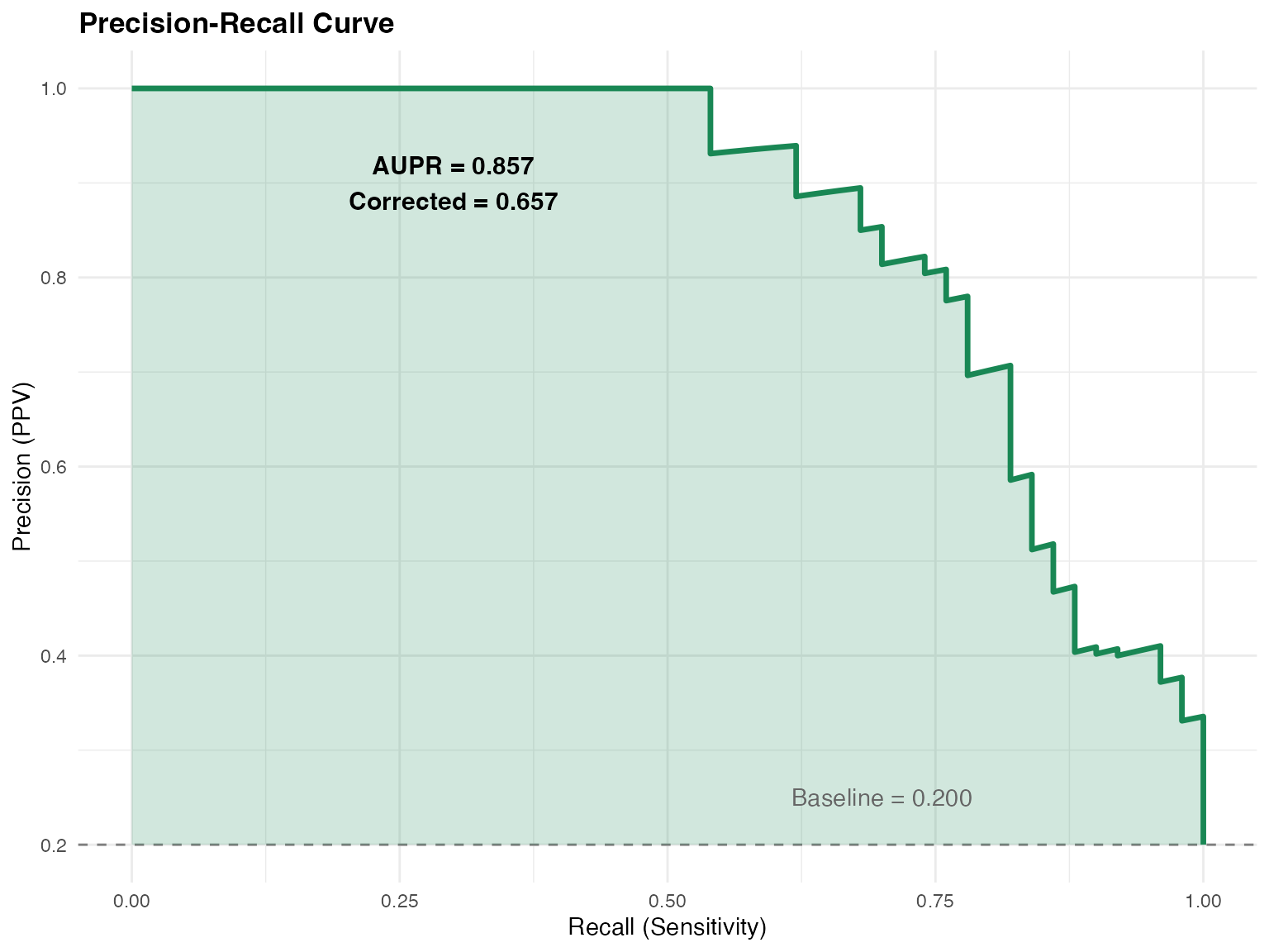

Precision-Recall curve with baseline

Pearson Correlation

$r = \frac{\sum_g (m_g - \bar{m})(y_g - \bar{y})}{\sqrt{\sum_g (m_g - \bar{m})^2} \sqrt{\sum_g (y_g - \bar{y})^2}}$

Statistical test: Under $H_0: \rho = 0$ :

$t = r \sqrt{\frac{n-2}{1-r^2}} \sim t_{n-2}$

Numerical Implementation

Computational Considerations

Sparse Matrix Operations

For efficiency, NicheNet uses sparse matrix representations:

# Example sparse matrix
library(Matrix)

# Dense vs sparse storage
n <- 1000
sparsity <- 0.01

set.seed(789)
dense_mat <- matrix(0, n, n)
dense_mat[sample(n^2, n^2 * sparsity)] <- runif(n^2 * sparsity)

sparse_mat <- Matrix(dense_mat, sparse = TRUE)

cat("Dense matrix size:", format(object.size(dense_mat), units = "MB"), "\n")

## Dense matrix size: 7.6 Mb

cat("Sparse matrix size:", format(object.size(sparse_mat), units = "MB"), "\n")

## Sparse matrix size: 0.1 Mb

cat("Compression ratio:", round(as.numeric(object.size(dense_mat)) / 
                                 as.numeric(object.size(sparse_mat)), 1), "x\n")

## Compression ratio: 63.7 x

C++ Acceleration

Critical operations are implemented in C++ for performance:

Operation	R Time	C++ Time	Speedup
AUROC/AUPR	~100ms	~2ms	50x
Pearson batch	~50ms	~1ms	50x
Matrix subset	~20ms	~0.5ms	40x

Numerical Stability

To prevent numerical issues:

Log-space operations for very small probabilities
Epsilon thresholds for division (default: $10^{-10}$ )
P-value capping at machine precision limit

Summary

The NicheNet algorithm combines:

Multi-source network integration with weighted aggregation
Hub-corrected adjacency matrices to prevent degree bias
Personalized PageRank for ligand-target scoring
Robust statistical evaluation using AUROC, AUPR, and correlation

This mathematical framework enables principled inference of intercellular signaling from transcriptomic data.

References

Browaeys R, Saelens W, Saeys Y. NicheNet: modeling intercellular communication by linking ligands to target genes. Nature Methods 17, 159–162 (2020).
Haveliwala TH. Topic-sensitive PageRank. WWW ’02: Proceedings of the 11th International Conference on World Wide Web (2002).
Davis J, Goadrich M. The relationship between Precision-Recall and ROC curves. ICML ’06 (2006).

Session Info

sessionInfo()

## R version 4.4.0 (2024-04-24)
## Platform: aarch64-apple-darwin20
## Running under: macOS 15.6.1
## 
## Matrix products: default
## BLAS:   /Library/Frameworks/R.framework/Versions/4.4-arm64/Resources/lib/libRblas.0.dylib 
## LAPACK: /Library/Frameworks/R.framework/Versions/4.4-arm64/Resources/lib/libRlapack.dylib;  LAPACK version 3.12.0
## 
## locale:
## [1] C
## 
## time zone: Asia/Shanghai
## tzcode source: internal
## 
## attached base packages:
## [1] stats     graphics  grDevices utils     datasets  methods   base     
## 
## other attached packages:
## [1] Matrix_1.7-4  tidyr_1.3.2   dplyr_1.1.4   ggplot2_4.0.1
## 
## loaded via a namespace (and not attached):
##  [1] gtable_0.3.6       jsonlite_2.0.0     compiler_4.4.0     tidyselect_1.2.1  
##  [5] dichromat_2.0-0.1  jquerylib_0.1.4    systemfonts_1.3.1  scales_1.4.0      
##  [9] textshaping_1.0.4  yaml_2.3.12        fastmap_1.2.0      lattice_0.22-7    
## [13] R6_2.6.1           labeling_0.4.3     generics_0.1.4     knitr_1.51        
## [17] htmlwidgets_1.6.4  tibble_3.3.1       desc_1.4.3         bslib_0.9.0       
## [21] pillar_1.11.1      RColorBrewer_1.1-3 rlang_1.1.7        cachem_1.1.0      
## [25] xfun_0.56          fs_1.6.6           sass_0.4.10        S7_0.2.1          
## [29] otel_0.2.0         viridisLite_0.4.2  cli_3.6.5          pkgdown_2.1.3     
## [33] withr_3.0.2        magrittr_2.0.4     digest_0.6.39      grid_4.4.0        
## [37] lifecycle_1.0.5    vctrs_0.7.0        evaluate_1.0.5     glue_1.8.0        
## [41] farver_2.1.2       ragg_1.5.0         purrr_1.2.1        rmarkdown_2.30    
## [45] tools_4.4.0        pkgconfig_2.0.3    htmltools_0.5.9

Zaoqu Liu, Robin Browaeys, Wouter Saelens, Yvan Saeys

2026-01-24