COMMOTR: Algorithm Theory and Mathematical Foundation
Zaoqu Liu
2026-01-25
Source:vignettes/algorithm_theory.Rmd
algorithm_theory.RmdIntroduction
COMMOTR implements collective optimal transport (COT) for inferring spatially-resolved cell-cell communication (CCC) in spatial transcriptomics data. This vignette provides a comprehensive overview of the mathematical foundations underlying the algorithm.
The Cell-Cell Communication Problem
Traditional Approaches
Traditional CCC inference methods typically compute a score for each cell pair based on:
However, this approach ignores spatial constraints — cells that are far apart are unlikely to communicate directly.
The Optimal Transport Formulation
COMMOTR formulates CCC as an optimal transport (OT) problem. Given:
- Source distribution : Ligand expression across cells
- Target distribution : Receptor expression across cells
- Cost matrix : Spatial distances between cells
The goal is to find a transport plan that optimally transports ligand signals to receptor locations.
Mathematical Formulation
Classical Optimal Transport (Kantorovich Problem)
The classical OT problem seeks:
where is the total transport cost.
Entropy-Regularized OT
Direct solution is computationally expensive (). Adding entropy regularization:
where:
This enables efficient solutions via the Sinkhorn-Knopp algorithm.
Unbalanced Optimal Transport
In CCC, total ligand production may not equal total receptor capacity. COMMOTR uses unbalanced OT with KL divergence penalties:
Key parameters:
| Parameter | Symbol | Role |
|---|---|---|
| Entropy regularization | Controls transport smoothness | |
| Unbalanced penalty | Controls mass conservation strictness |
The Sinkhorn Algorithm
Collective Optimal Transport
Communication Direction
Visualization Example
library(ggplot2)

# Simulate transport problem
set.seed(42)
n <- 20
x <- runif(n, 0, 100)
y <- runif(n, 0, 100)
coords <- data.frame(x = x, y = y,
                    type = rep(c("Sender", "Receiver"), each = n/2))

# Create distance-based cost
dist_mat <- as.matrix(dist(coords[, c("x", "y")]))

# Visualize cost matrix
cost_df <- expand.grid(i = 1:n, j = 1:n)
cost_df$distance <- as.vector(dist_mat)
cost_df$cost <- ifelse(cost_df$distance < 50, cost_df$distance / 50, NA)

p1 <- ggplot(cost_df, aes(x = i, y = j, fill = cost)) +
  geom_tile() +
  scale_fill_viridis_c(na.value = "white", name = "Cost") +
  labs(title = "Distance-Based Cost Matrix",
       subtitle = "White = beyond threshold (infinite cost)",
       x = "Source cell", y = "Target cell") +
  coord_fixed() +
  theme_minimal()

print(p1)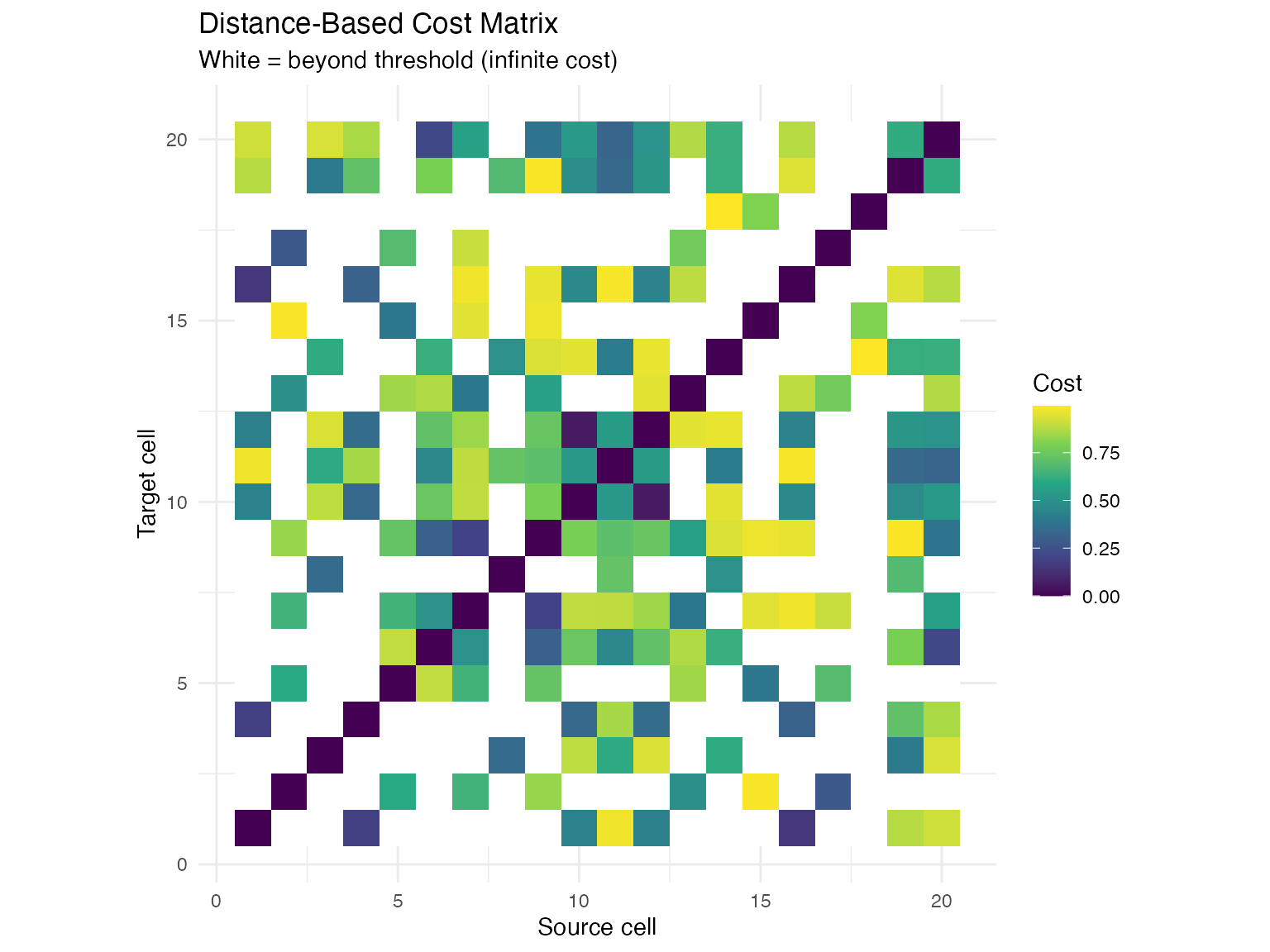
# Visualize simulated transport
# (Simplified for demonstration)
senders <- coords[1:10, ]
receivers <- coords[11:20, ]

# Create transport connections (top pairs)
set.seed(123)
connections <- data.frame(
  x_start = senders$x[sample(10, 15, replace = TRUE)],
  y_start = senders$y[sample(10, 15, replace = TRUE)],
  x_end = receivers$x[sample(10, 15, replace = TRUE)],
  y_end = receivers$y[sample(10, 15, replace = TRUE)],
  weight = runif(15, 0.1, 1)
)

p2 <- ggplot() +
  geom_segment(data = connections,
               aes(x = x_start, y = y_start, xend = x_end, yend = y_end,
                   alpha = weight, linewidth = weight),
               color = "#E63946",
               arrow = arrow(length = unit(0.15, "cm"))) +
  geom_point(data = senders, aes(x = x, y = y),
             color = "#1D3557", size = 4, shape = 16) +
  geom_point(data = receivers, aes(x = x, y = y),
             color = "#457B9D", size = 4, shape = 17) +
  scale_alpha_continuous(range = c(0.3, 0.9), guide = "none") +
  scale_linewidth_continuous(range = c(0.3, 1.5), guide = "none") +
  labs(title = "Optimal Transport Plan Visualization",
       subtitle = "Arrows show ligand→receptor transport (width = intensity)",
       x = "Spatial X", y = "Spatial Y") +
  annotate("text", x = 90, y = 95, label = "● Sender", hjust = 0, size = 3) +
  annotate("text", x = 90, y = 88, label = "▲ Receiver", hjust = 0, size = 3) +
  theme_minimal() +
  coord_fixed()

print(p2)![]()
Parameter Selection Guide
# Illustrate effect of epsilon and rho
params <- expand.grid(
  eps = c(0.01, 0.1, 1.0),
  rho = c(1, 10, 100)
)
params$smoothness <- 1 / params$eps
params$balance <- params$rho / (params$rho + 1)

ggplot(params, aes(x = eps, y = rho)) +
  geom_tile(aes(fill = balance), color = "white", linewidth = 1) +
  geom_text(aes(label = sprintf("ε=%.2f\nρ=%d", eps, rho)),
            size = 3, color = "white") +
  scale_fill_gradient(low = "#457B9D", high = "#E63946",
                     name = "Mass\nConservation") +
  scale_x_log10() + scale_y_log10() +
  labs(title = "Parameter Space Overview",
       subtitle = "ε: entropy regularization | ρ: unbalanced penalty",
       x = "Entropy (ε) - log scale",
       y = "Unbalanced penalty (ρ) - log scale") +
  theme_minimal()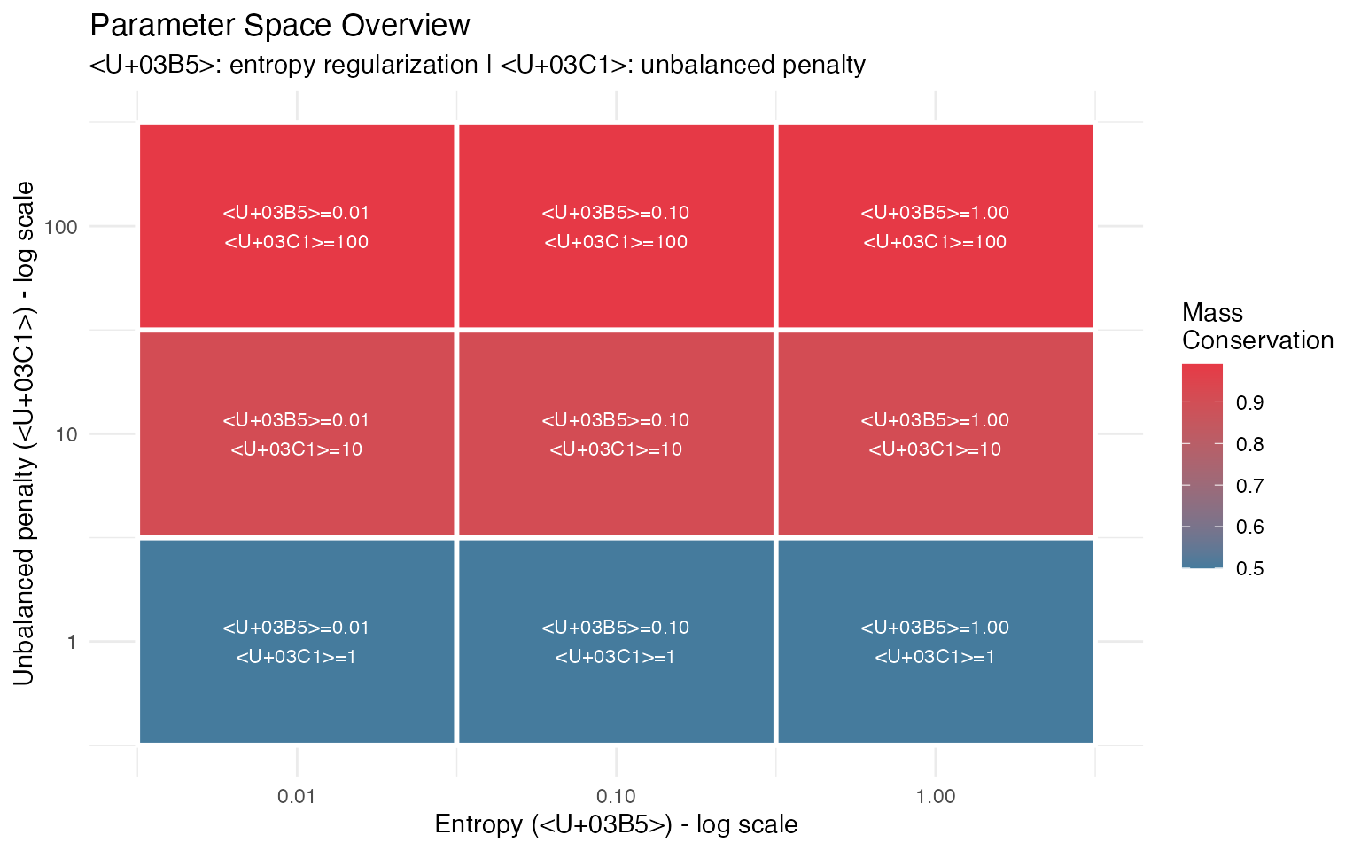
References
Cang, Z., Zhao, Y., et al. Screening cell–cell communication in spatial transcriptomics via collective optimal transport. Nature Methods 20, 218–228 (2023).
Cuturi, M. Sinkhorn Distances: Lightspeed Computation of Optimal Transport. NeurIPS (2013).
Chizat, L., et al. Scaling algorithms for unbalanced optimal transport problems. Mathematics of Computation 87, 2563–2609 (2018).
Developed by Zaoqu Liu | GitHub | liuzaoqu@163.com