Quick Start Guide

Overview

This guide demonstrates the essential COMMOTR workflow in 5 simple steps: 1. Load ligand-receptor database 2. Infer spatial communication 3. Compute communication direction 4. Analyze cluster communication 5. Visualize results

Installation

# From R-universe (recommended)
install.packages("COMMOTR", repos = "https://zaoqu-liu.r-universe.dev")

# From GitHub
remotes::install_github("Zaoqu-Liu/COMMOTR")

Setup

library(COMMOTR)
library(Seurat)
library(Matrix)
library(ggplot2)

Create Demo Data

For this tutorial, we create a simulated spatial dataset with known communication patterns:

set.seed(42)

# Simulate 100 cells in two spatial clusters
n_cells <- 100
n_genes <- 50

# Create expression matrix
expr <- matrix(rpois(n_cells * n_genes, lambda = 5), 
               nrow = n_genes, ncol = n_cells)

# Gene names including ligand-receptor pairs
gene_names <- c("Tgfb1", "Tgfbr1", "Tgfbr2",  # TGFb pathway
                "Wnt5a", "Fzd1", "Lrp5",       # Wnt pathway
                "Fgf2", "Fgfr1",               # FGF pathway
                paste0("Gene", 1:(n_genes - 8)))
rownames(expr) <- gene_names
colnames(expr) <- paste0("Cell", 1:n_cells)

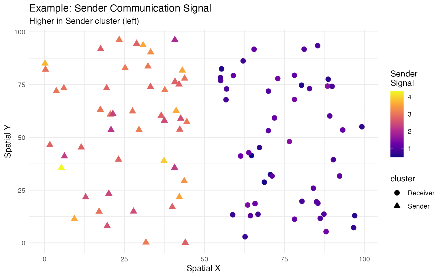
# Create spatial structure: left cluster (ligand-high), right cluster (receptor-high)
coords <- matrix(c(
  runif(50, 0, 45),   runif(50, 55, 100),  # x coordinates
  runif(100, 0, 100)                        # y coordinates
), ncol = 2)
rownames(coords) <- colnames(expr)
colnames(coords) <- c("x", "y")

# Add differential expression
expr["Tgfb1", 1:50] <- expr["Tgfb1", 1:50] + 15
expr["Tgfbr1", 51:100] <- expr["Tgfbr1", 51:100] + 15
expr["Tgfbr2", 51:100] <- expr["Tgfbr2", 51:100] + 15

# Create Seurat object
seurat_obj <- CreateSeuratObject(counts = expr, assay = "RNA")
seurat_obj <- SetAssayData(seurat_obj, layer = "data", 
                           new.data = log1p(as(expr, "dgCMatrix")))

# Add spatial coordinates
colnames(coords) <- c("spatial_1", "spatial_2")
seurat_obj[["spatial"]] <- CreateDimReducObject(
  embeddings = coords, key = "spatial_", assay = "RNA"
)

# Add cluster labels
seurat_obj$cluster <- factor(c(rep("Sender", 50), rep("Receiver", 50)))

Step 1: Load LR Database

# Create custom LR database for demo
df_lr <- data.frame(
  ligand = c("Tgfb1", "Wnt5a", "Fgf2"),
  receptor = c("Tgfbr1_Tgfbr2", "Fzd1_Lrp5", "Fgfr1"),
  pathway = c("TGFb", "WNT", "FGF"),
  stringsAsFactors = FALSE
)

# In real analysis, load from built-in databases:
df_lr <- ligand_receptor_database("CellChat", "mouse", "Secreted Signaling")
df_lr <- filter_lr_database(df_lr, seurat_obj, min_cell_pct = 0.05)

Step 2: Infer Spatial Communication

# Run spatial communication inference
seurat_obj <- spatial_communication(
  seurat_obj,
  df_ligrec = df_lr,
  database_name = "demo",
  spatial_coords = "spatial",
  dis_thr = 40,           # Distance threshold
  cot_eps_p = 0.1,        # Entropy regularization
  cot_rho = 10,           # Unbalanced penalty
  verbose = TRUE
)

# Access results
results <- get_communication_results(seurat_obj, "demo")

Step 3: Communication Direction

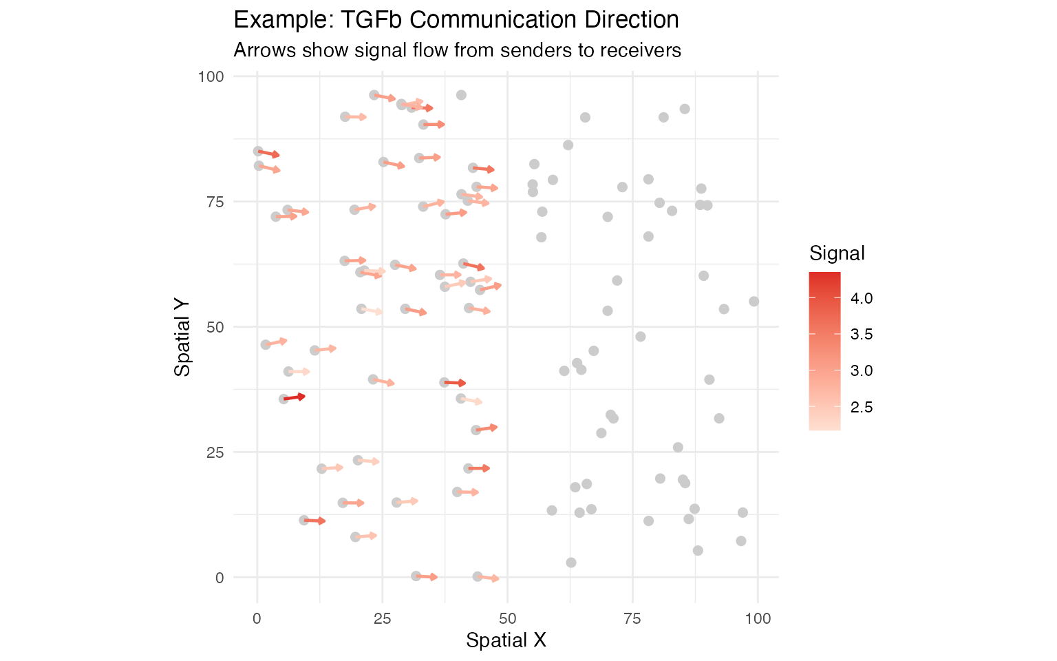
# Compute vector field for TGFb pathway
seurat_obj <- communication_direction(
  seurat_obj,
  database_name = "demo",
  pathway_name = "TGFb",
  spatial_coords = "spatial",
  k = 5
)

Step 4: Cluster Communication

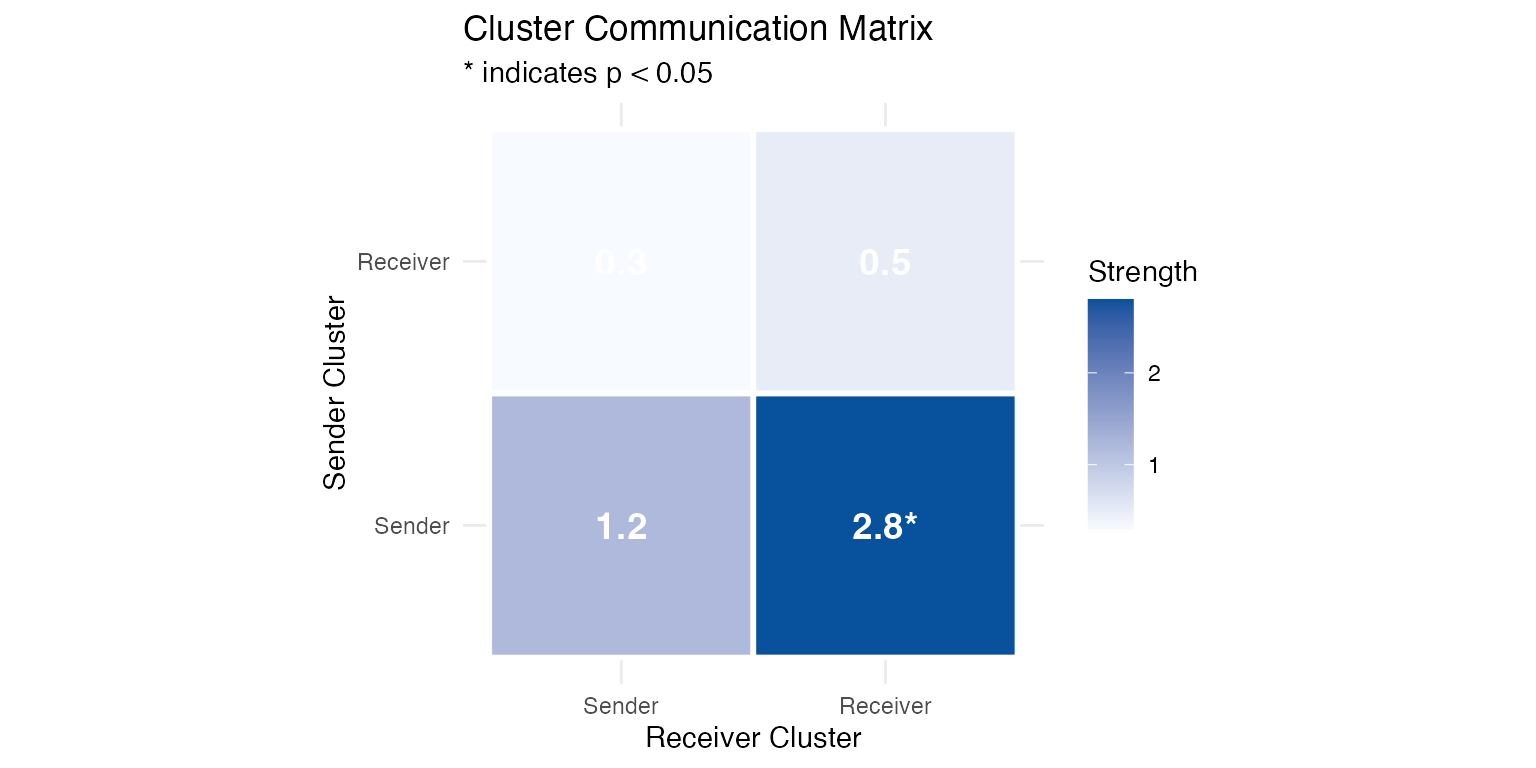
# Analyze cluster-level communication with permutation test
seurat_obj <- cluster_communication(
  seurat_obj,
  database_name = "demo",
  clustering = "cluster",
  pathway_name = "TGFb",
  n_permutations = 100
)

Step 5: Visualization

Spatial Communication Plot

Vector Field Visualization

Cluster Communication Heatmap

Summary

Step	Function	Purpose
1	`ligand_receptor_database()`	Load LR pairs
2	`spatial_communication()`	Infer communication
3	`communication_direction()`	Compute vector fields
4	`cluster_communication()`	Cluster-level analysis
5	Visualization	Interpret results

Next Steps

Read the Algorithm Theory vignette for mathematical details
Explore the Visualization Gallery for more plot types
Check the Full Tutorial for advanced analysis

Developed by Zaoqu Liu | GitHub | liuzaoqu@163.com

Zaoqu Liu

2026-01-25