Algorithm Details and Mathematical Framework

Mathematical Framework

This vignette provides a detailed description of the mathematical foundations underlying the MultiK algorithm.

1. Consensus Clustering

1.1 Subsampling Strategy

Given a dataset with $N$ cells, MultiK performs $R$ subsampling iterations. In each iteration $r$ :

Randomly sample $\lfloor p \cdot N \rfloor$ cells without replacement (default $p = 0.8$ )
Apply the standard Seurat clustering pipeline across $M$ resolution parameters

1.2 Consensus Matrix Construction

For each cluster number $K$ , we construct a consensus matrix $\mathbf{C}^{(K)} \in [0,1]^{N \times N}$ :

$C_{ij}^{(K)} = \frac{\sum_{r=1}^{R_K} \mathbf{1}[\text{cell } i \text{ and } j \text{ co-cluster in run } r]}{\sum_{r=1}^{R_K} \mathbf{1}[\text{cell } i \text{ and } j \text{ co-sampled in run } r]}$

where $R_K$ is the number of runs that yielded exactly $K$ clusters.

Properties of the consensus matrix:

$C_{ii} = 1$ (a cell always co-clusters with itself)
$C_{ij} = C_{ji}$ (symmetric)
$C_{ij} \in [0, 1]$
$C_{ij} = 1$ implies cells $i$ and $j$ always cluster together
$C_{ij} = 0$ implies cells never cluster together

1.3 Visualizing the Consensus Matrix

library(ggplot2)

# Simulate a consensus matrix with 3 clear clusters
set.seed(42)
n <- 60
blocks <- c(rep(1, 20), rep(2, 20), rep(3, 20))

mat <- matrix(0, n, n)
for (i in 1:n) {
  for (j in 1:n) {
    if (blocks[i] == blocks[j]) {
      mat[i, j] <- runif(1, 0.85, 1.0)
    } else {
      mat[i, j] <- runif(1, 0, 0.15)
    }
  }
}
diag(mat) <- 1
mat[lower.tri(mat)] <- t(mat)[lower.tri(mat)]

# Reorder by cluster
ord <- order(blocks)
mat_ord <- mat[ord, ord]

df_cons <- expand.grid(Cell1 = 1:n, Cell2 = 1:n)
df_cons$value <- as.vector(mat_ord)

ggplot(df_cons, aes(x = Cell1, y = Cell2, fill = value)) +
  geom_tile() +
  scale_fill_gradient2(low = "#3498DB", mid = "white", high = "#E74C3C",
                       midpoint = 0.5, limits = c(0, 1),
                       name = "Co-clustering\nProbability") +
  labs(x = "Cell Index", y = "Cell Index",
       title = "Consensus Matrix Heatmap",
       subtitle = "Clear block structure indicates stable clusters") +
  coord_fixed() +
  theme_minimal(base_size = 12) +
  theme(plot.title = element_text(face = "bold"),
        panel.grid = element_blank())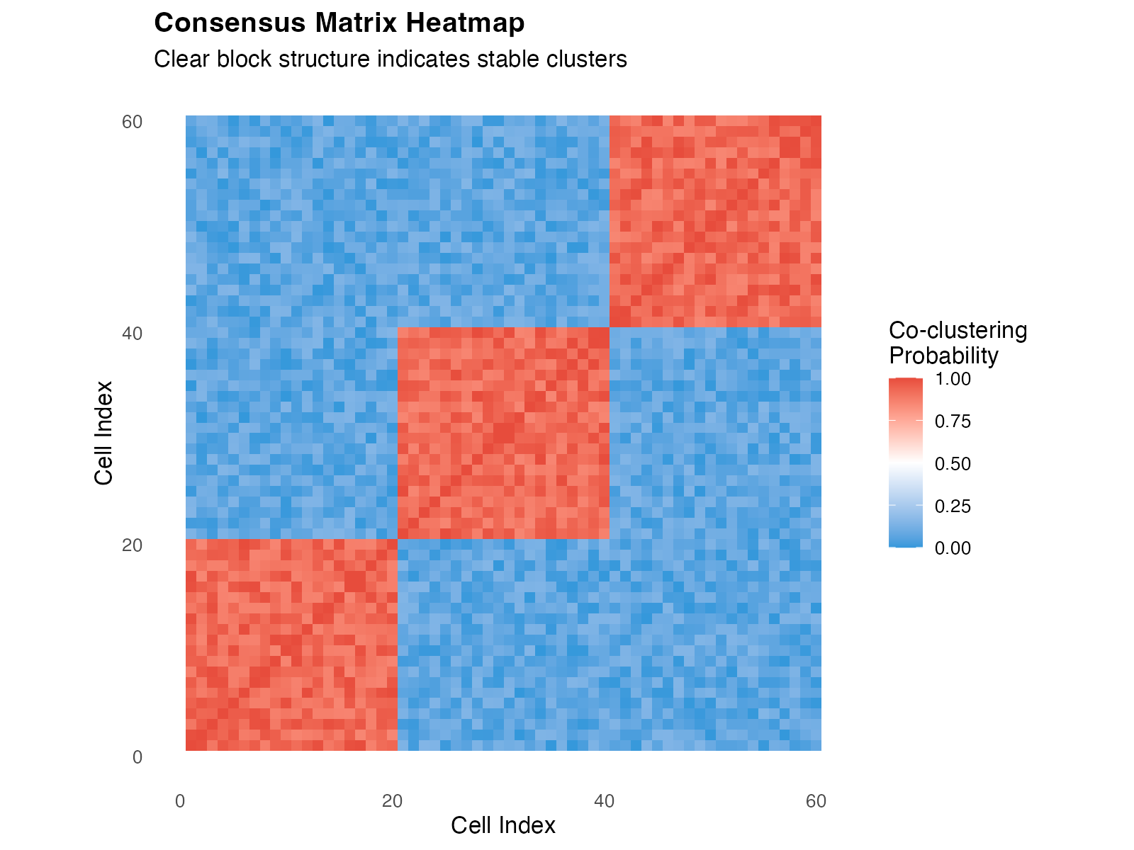

Example consensus matrix showing clear block-diagonal structure indicating well-separated clusters.

2. Proportion of Ambiguous Clustering (PAC)

2.1 Definition

The PAC metric quantifies clustering ambiguity by measuring the proportion of cell pairs with intermediate consensus values:

$\text{PAC}(K) = \frac{|\{(i,j): x_1 < C_{ij}^{(K)} < x_2, i < j\}|}{|\{(i,j): i < j\}|}$

where $x_1 = 0.1$ and $x_2 = 0.9$ are default thresholds.

2.2 Interpretation

PAC Value	Interpretation
PAC ≈ 0	Clear cluster structure, cells consistently assigned
PAC ≈ 1	Ambiguous clustering, unstable cell assignments

2.3 PAC Visualization

# Simulate PAC values for different K
df_pac <- data.frame(
  K = factor(2:8),
  PAC = c(0.12, 0.05, 0.08, 0.18, 0.35, 0.52, 0.68)
)
df_pac$rPAC <- df_pac$PAC / max(df_pac$PAC)

p1 <- ggplot(df_pac, aes(x = K, y = PAC)) +
  geom_col(fill = "#3498DB", color = "black", width = 0.7) +
  geom_hline(yintercept = 0.1, linetype = "dashed", color = "red") +
  labs(x = "Number of Clusters (K)", y = "PAC",
       title = "Absolute PAC") +
  theme_bw(base_size = 12) +
  theme(plot.title = element_text(face = "bold"))

p2 <- ggplot(df_pac, aes(x = K, y = rPAC)) +
  geom_col(fill = "#E74C3C", color = "black", width = 0.7) +
  labs(x = "Number of Clusters (K)", y = "Relative PAC (rPAC)",
       title = "Relative PAC (normalized)") +
  theme_bw(base_size = 12) +
  theme(plot.title = element_text(face = "bold"))

cowplot::plot_grid(p1, p2, ncol = 2)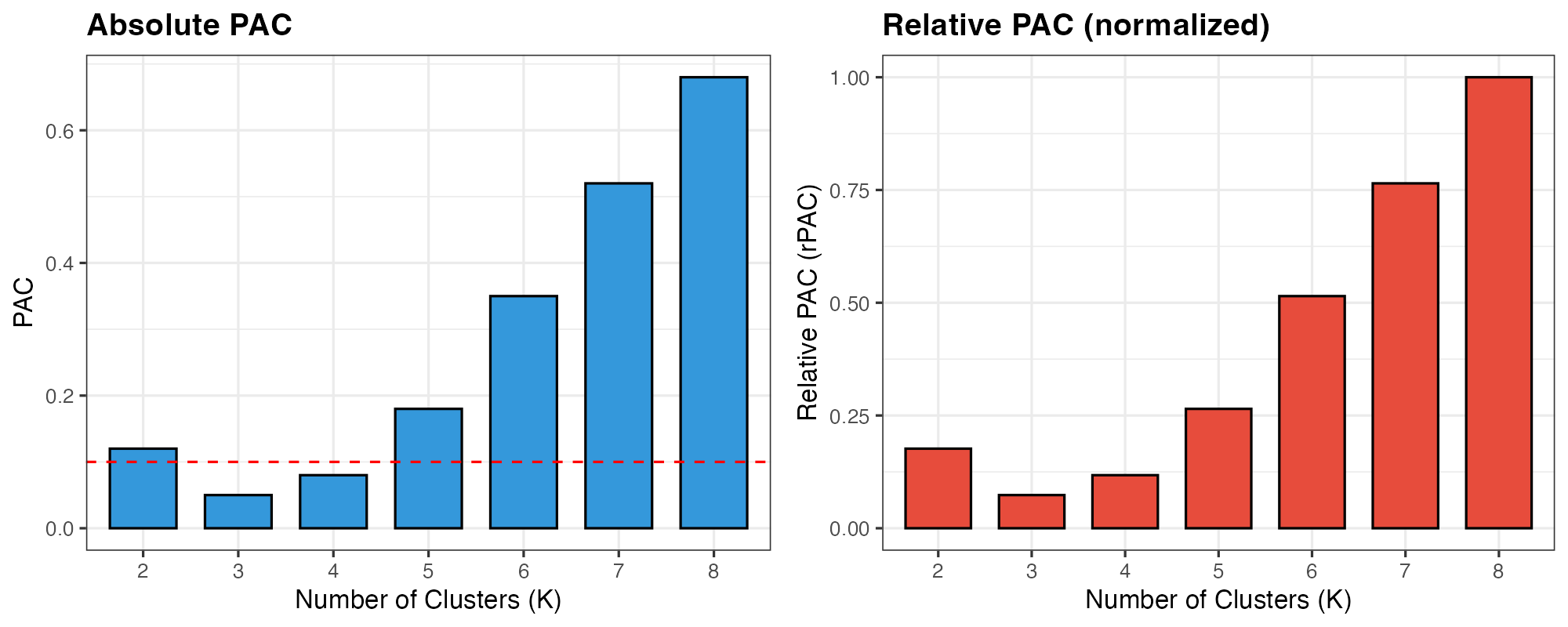

PAC values across different K. Lower PAC indicates more stable clustering.

2.4 Relative PAC (rPAC)

To enable comparison across different K values:

$\text{rPAC}(K) = \frac{\text{PAC}(K)}{\max_k \text{PAC}(k)}$

Lower rPAC indicates more stable clustering.

3. Optimal K Selection

3.1 Multi-Objective Optimization

Optimal K should satisfy two criteria:

High frequency: K appears consistently across resolution parameters
Low rPAC: Clustering is stable (low ambiguity)

3.2 Pareto Frontier

We identify optimal K values using Pareto optimality. A point $(x_i, y_i)$ is Pareto-optimal if no other point $(x_j, y_j)$ satisfies:

$x_j \geq x_i \text{ and } y_j \geq y_i \text{ with at least one strict inequality}$

where: - $x = 1 - \text{rPAC}$ (stability) - $y = \text{frequency}$

set.seed(42)
df <- data.frame(
  K = factor(2:8),
  stability = c(0.88, 0.95, 0.92, 0.82, 0.65, 0.48, 0.32),
  frequency = c(25, 120, 85, 95, 110, 75, 40)
)

# Find Pareto optimal points
pareto <- c()
for (i in 1:nrow(df)) {
  dominated <- FALSE
  for (j in 1:nrow(df)) {
    if (i != j) {
      if (df$stability[j] >= df$stability[i] && df$frequency[j] >= df$frequency[i] &&
          (df$stability[j] > df$stability[i] || df$frequency[j] > df$frequency[i])) {
        dominated <- TRUE
        break
      }
    }
  }
  if (!dominated) pareto <- c(pareto, i)
}

df$optimal <- 1:7 %in% pareto

ggplot(df, aes(x = stability, y = frequency)) +
  geom_point(aes(color = optimal), size = 5) +
  geom_text(aes(label = paste0("K=", K)), vjust = -1.2, size = 4) +
  scale_color_manual(values = c("FALSE" = "gray50", "TRUE" = "#E74C3C"), 
                     guide = "none") +
  geom_vline(xintercept = 0.9, linetype = "dashed", alpha = 0.5) +
  geom_hline(yintercept = 100, linetype = "dashed", alpha = 0.5) +
  annotate("rect", xmin = 0.9, xmax = 1, ymin = 100, ymax = 130, 
           fill = "green", alpha = 0.1) +
  annotate("text", x = 0.95, y = 125, label = "Ideal\nRegion", size = 3) +
  labs(x = "Stability (1 - rPAC)", y = "Frequency",
       title = "Pareto Frontier for Optimal K Selection",
       subtitle = "Red points = Pareto-optimal; Green region = ideal") +
  xlim(0.25, 1) +
  theme_bw(base_size = 12) +
  theme(plot.title = element_text(face = "bold"))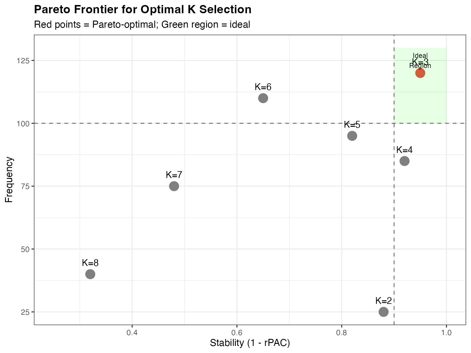

Pareto frontier for K selection. Red points indicate Pareto-optimal K values.

4. SigClust Statistical Testing

4.1 Hypothesis Framework

For each pair of clusters $C_a$ and $C_b$ , SigClust tests:

$H_0$ : Data come from a single Gaussian distribution
$H_1$ : Data come from two distinct distributions

4.2 Cluster Index

The test statistic is the cluster index (CI):

$\text{CI} = \frac{2 \cdot n_a \cdot n_b}{(n_a + n_b)^2} \cdot \frac{\|\bar{x}_a - \bar{x}_b\|^2}{\text{tr}(\hat{\Sigma})}$

where: - $n_a, n_b$ are cluster sizes - $\bar{x}_a, \bar{x}_b$ are cluster centroids - $\hat{\Sigma}$ is the pooled covariance estimate

4.3 P-value Heatmap Interpretation

# Create example p-value matrix
pval_mat <- matrix(c(NA, 0.001, 0.015, 0.042,
                     0.001, NA, 0.003, 0.089,
                     0.015, 0.003, NA, 0.008,
                     0.042, 0.089, 0.008, NA), 4, 4, byrow = TRUE)
rownames(pval_mat) <- colnames(pval_mat) <- paste0("Cluster", 1:4)

df_heat <- expand.grid(Cluster1 = rownames(pval_mat), 
                       Cluster2 = colnames(pval_mat))
df_heat$pvalue <- as.vector(pval_mat)

ggplot(df_heat, aes(x = Cluster1, y = Cluster2, fill = pvalue)) +
  geom_tile(color = "white", linewidth = 1) +
  geom_text(aes(label = ifelse(is.na(pvalue), "", sprintf("%.3f", pvalue))), 
            size = 5, fontface = "bold") +
  scale_fill_gradient2(low = "#27AE60", mid = "#F1C40F", high = "#E74C3C",
                       midpoint = 0.05, limits = c(0, 0.1),
                       na.value = "grey90",
                       name = "P-value") +
  labs(x = "", y = "",
       title = "Pairwise SigClust P-values",
       subtitle = "Green (p < 0.05) = significant separation") +
  coord_fixed() +
  theme_minimal(base_size = 12) +
  theme(plot.title = element_text(face = "bold"),
        panel.grid = element_blank(),
        axis.text = element_text(size = 11, face = "bold"))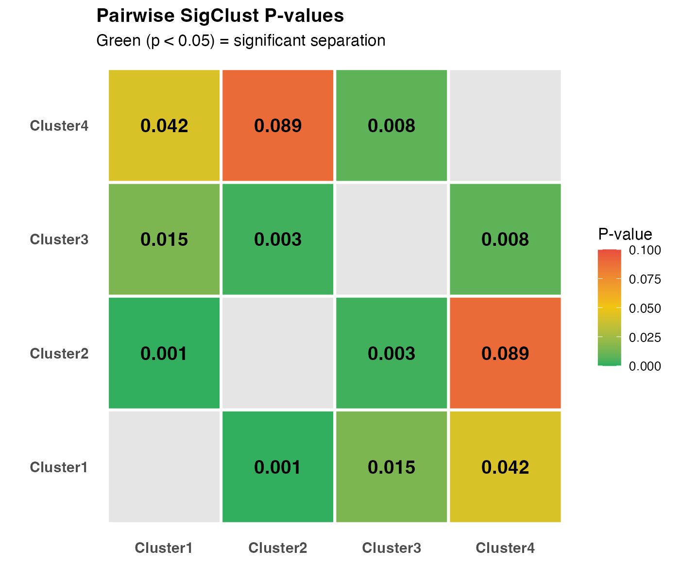

Pairwise SigClust p-value heatmap. Green indicates significant separation.

4.4 Interpretation Guide

P-value	Interpretation	Action
$p < 0.01$	Highly significant separation	Distinct clusters
$0.01 \leq p < 0.05$	Significant separation	Likely distinct
$0.05 \leq p < 0.10$	Borderline	Consider merging
$p \geq 0.10$	Not significant	May be subclasses

5. Complete Workflow Visualization

library(ggplot2)

# Create workflow diagram
steps <- data.frame(
  x = 1:5,
  y = rep(0, 5),
  label = c("1. Input\nSeurat Object", 
            "2. Subsampling\n& Clustering",
            "3. Consensus\nMatrix",
            "4. PAC &\nOptimal K",
            "5. SigClust\nValidation"),
  color = c("#3498DB", "#9B59B6", "#E74C3C", "#F1C40F", "#27AE60")
)

ggplot(steps, aes(x = x, y = y)) +
  geom_segment(aes(x = 1.3, xend = 4.7, y = 0, yend = 0),
               arrow = arrow(length = unit(0.3, "cm"), type = "closed"),
               color = "gray40", linewidth = 1.5) +
  geom_point(aes(fill = color), shape = 21, size = 20, color = "black", stroke = 2) +
  geom_text(aes(label = label), y = -0.15, size = 3.5, lineheight = 0.9) +
  scale_fill_identity() +
  coord_cartesian(ylim = c(-0.3, 0.15), xlim = c(0.5, 5.5)) +
  theme_void() +
  labs(title = "MultiK Analysis Workflow") +
  theme(plot.title = element_text(hjust = 0.5, face = "bold", size = 14))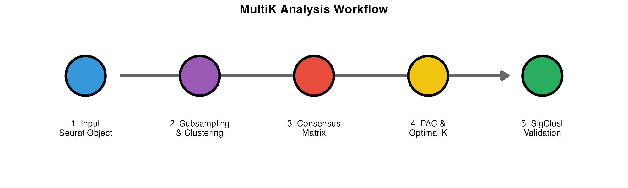

MultiK analysis workflow.

6. Computational Complexity

Component	Complexity
Single clustering run	$O(N \log N)$
All subsampling iterations	$O(R \cdot M \cdot N \log N)$
Consensus matrix	$O(R_K \cdot N^2)$
PAC calculation	$O(N^2)$
SigClust (per pair)	$O(B \cdot n_k^2)$

where $N$ = cells, $R$ = reps, $M$ = resolutions, $B$ = simulations.

7. Parameter Recommendations

Parameter	Recommended	Rationale
`reps`	100-200	Sufficient for stable consensus
`pSample`	0.8	Balance between variation and representation
`resolution`	0.05-2.0	Covers typical cluster range
`nsim`	100-500	Accurate p-value estimation

References

Consensus Clustering: Monti S, et al. (2003) Consensus Clustering. Machine Learning 52:91-118.
PAC Metric: Șenbabaoğlu Y, et al. (2014) Critical limitations of consensus clustering. Scientific Reports 4:6207.
SigClust: Liu Y, et al. (2008) Statistical significance of clustering. JASA 103:1281-1293.

Author

Zaoqu Liu, PhD

Email: liuzaoqu@163.com
ORCID: 0000-0002-0452-742X

This vignette is part of the MultiK package. For questions or issues, please visit GitHub.

Zaoqu Liu

2026-01-23