Introduction to MultiK
Zaoqu Liu
2026-01-23
Source:vignettes/MultiK-introduction.Rmd
MultiK-introduction.RmdOverview
MultiK is a computational framework for objective determination of optimal cluster numbers in single-cell RNA sequencing (scRNA-seq) data. Selecting the appropriate number of clusters (K) is a fundamental challenge in unsupervised clustering analysis, and MultiK addresses this through a rigorous statistical approach.
The Challenge
In scRNA-seq analysis, researchers often face the question: “How many distinct cell populations exist in my data?” Traditional approaches rely on:
- Arbitrary selection based on visualization
- Rule-of-thumb methods (e.g., elbow method)
- Biological prior knowledge
These approaches are subjective and may miss important biological structures or over-partition the data.
Installation
# From R-universe (recommended)
install.packages("MultiK", repos = "https://zaoqu-liu.r-universe.dev")

# From GitHub
remotes::install_github("Zaoqu-Liu/MultiK")
Quick Start
Load Package and Data
library(MultiK)
library(Seurat)
library(ggplot2)

# Load example data
data(p3cl)
p3cl
#> An object of class Seurat
#> 21247 features across 2609 samples within 1 assay
#> Active assay: RNA (21247 features, 0 variable features)
The p3cl dataset contains approximately 2,600 cells from
a three cell line mixture (H2228, H1975, HCC827), providing a benchmark
with known ground truth (K=3).
Step 1: Run MultiK Algorithm
# Run with 50 subsampling iterations (use 100+ for production)
set.seed(42)
result <- MultiK(p3cl,
                 reps = 50,
                 resolution = seq(0.1, 1.5, 0.1),
                 nPC = 20,
                 cores = 1,
                 seed = 42)

# Check the distribution of K values
table(result$k)
#>
#>  3  4  5  6  7  8  9 10 11 12 13 14 15 16
#> 52 65 63 96 70 68 79 71 71 64 33 13  4  1
Step 2: Diagnostic Visualization
# Generate diagnostic plots
DiagMultiKPlot(result$k, result$consensus)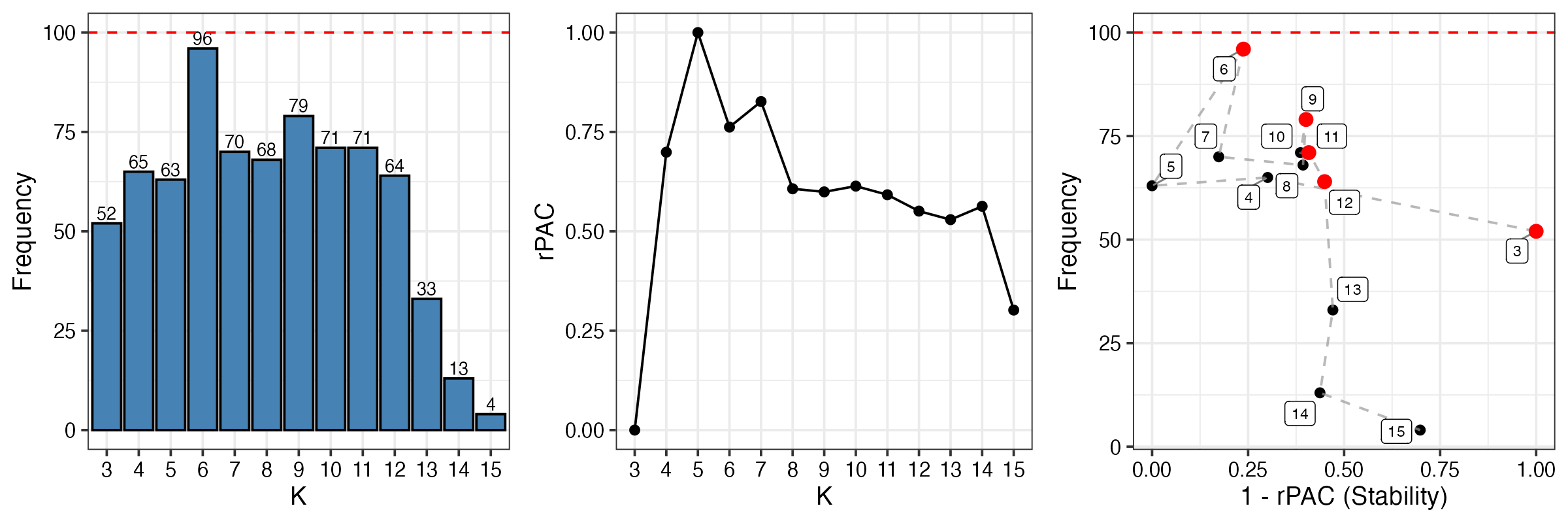
Interpretation of diagnostic plots:
- Left panel (Frequency): Shows how often each K value was observed across all clustering runs. K=3 appears most frequently, suggesting it’s a stable solution.
- Middle panel (rPAC): Relative PAC scores for each K. Lower values indicate more stable clustering. K=3 shows low rPAC.
- Right panel (Trade-off): Combines frequency and stability. Points in the upper-right corner (high frequency, high stability) are optimal. The red point indicates the recommended K.
Step 3: Extract Clusters
# Get cluster assignments at optimal K=3
clusters <- getClusters(p3cl, optK = 3, nPC = 20)

# View cluster distribution
table(clusters$clusters[, 1])
#>
#>    0    1    2
#> 1854  541  214

# Add clusters to Seurat object for visualization
p3cl$multik_clusters <- factor(clusters$clusters[, 1])
Step 4: Visualize Clusters
# Run UMAP for visualization
p3cl <- NormalizeData(p3cl, verbose = FALSE)
p3cl <- FindVariableFeatures(p3cl, verbose = FALSE)
p3cl <- ScaleData(p3cl, verbose = FALSE)
p3cl <- RunPCA(p3cl, npcs = 20, verbose = FALSE)
p3cl <- RunUMAP(p3cl, dims = 1:20, verbose = FALSE)

# Plot UMAP with MultiK clusters
DimPlot(p3cl, group.by = "multik_clusters",
        cols = c("#E41A1C", "#377EB8", "#4DAF4A"),
        pt.size = 0.5) +
  ggtitle("MultiK Clustering (K=3)") +
  theme(plot.title = element_text(hjust = 0.5, face = "bold"))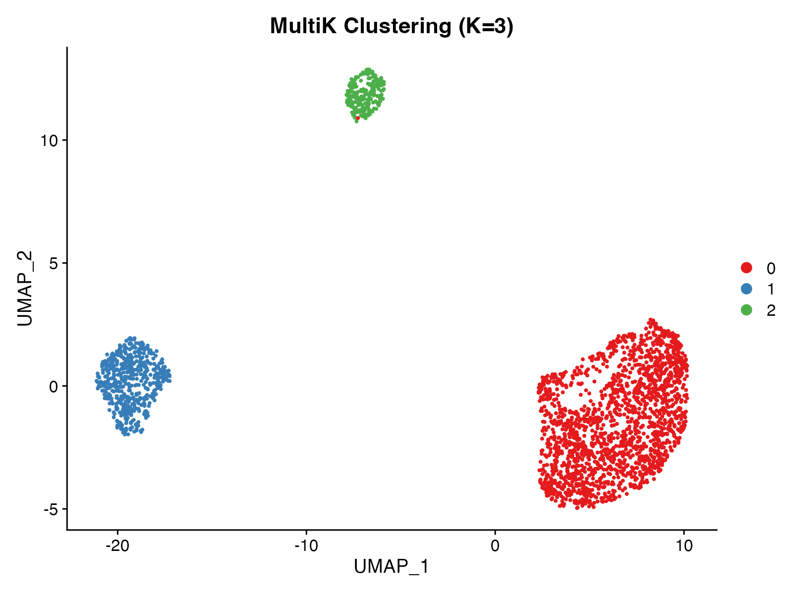
Step 5: Statistical Validation
# Pairwise SigClust tests
pval <- CalcSigClust(p3cl, clusters$clusters[, 1], nsim = 50, cores = 1)

# View p-value matrix
print(round(pval, 4))
#>          cluster0 cluster1 cluster2
#> cluster0       NA        0        0
#> cluster1        0       NA        0
#> cluster2        0        0       NA

# Visualize results
PlotSigClust(p3cl, clusters$clusters[, 1], pval)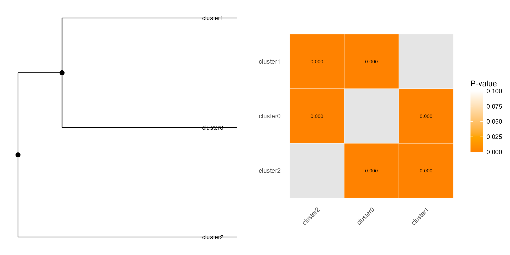
Interpretation:
- Dendrogram (left): Shows hierarchical relationships between clusters based on expression similarity
- Filled circles (●): All pairwise comparisons at this node are significant (p < 0.05) - true distinct clusters
- Open circles (○): At least one non-significant comparison - potential subclasses
- Heatmap (right): Pairwise p-values. Red/orange = significant separation, white = similar
In this example, all three clusters show significant separation (p < 0.05), confirming they represent distinct cell populations.
Key Functions
| Function | Purpose |
|---|---|
MultiK() |
Core consensus clustering algorithm |
DiagMultiKPlot() |
Diagnostic visualization for K selection |
getClusters() |
Extract cluster assignments |
CalcSigClust() |
Statistical significance testing |
PlotSigClust() |
Visualize cluster relationships |
Summary
MultiK provides a rigorous, data-driven approach to determine optimal cluster numbers:
- Run MultiK with multiple subsampling iterations
- Examine diagnostic plots to identify optimal K
- Extract clusters at the chosen K
- Validate with SigClust statistical testing
This workflow ensures reproducible and statistically justified clustering results.
Session Info
sessionInfo()
#> R version 4.4.0 (2024-04-24)
#> Platform: aarch64-apple-darwin20
#> Running under: macOS 15.6.1
#>
#> Matrix products: default
#> BLAS:   /Library/Frameworks/R.framework/Versions/4.4-arm64/Resources/lib/libRblas.0.dylib
#> LAPACK: /Library/Frameworks/R.framework/Versions/4.4-arm64/Resources/lib/libRlapack.dylib;  LAPACK version 3.12.0
#>
#> locale:
#> [1] C
#>
#> time zone: Asia/Shanghai
#> tzcode source: internal
#>
#> attached base packages:
#> [1] stats     graphics  grDevices utils     datasets  methods   base
#>
#> other attached packages:
#> [1] future_1.69.0      ggplot2_4.0.1      SeuratObject_4.1.4 Seurat_4.4.0
#> [5] MultiK_1.0.0
#>
#> loaded via a namespace (and not attached):
#>   [1] deldir_2.0-4           pbapply_1.7-4          gridExtra_2.3
#>   [4] rlang_1.1.7            magrittr_2.0.4         RcppAnnoy_0.0.23
#>   [7] otel_0.2.0             spatstat.geom_3.6-1    matrixStats_1.5.0
#>  [10] ggridges_0.5.7         compiler_4.4.0         png_0.1-8
#>  [13] systemfonts_1.3.1      vctrs_0.7.0            reshape2_1.4.5
#>  [16] stringr_1.6.0          pkgconfig_2.0.3        fastmap_1.2.0
#>  [19] labeling_0.4.3         promises_1.5.0         rmarkdown_2.30
#>  [22] ragg_1.5.0             purrr_1.2.1            xfun_0.56
#>  [25] cachem_1.1.0           sigclust_1.1.0.1       jsonlite_2.0.0
#>  [28] goftest_1.2-3          later_1.4.5            spatstat.utils_3.2-1
#>  [31] irlba_2.3.5.1          parallel_4.4.0         cluster_2.1.8.1
#>  [34] R6_2.6.1               ica_1.0-3              spatstat.data_3.1-9
#>  [37] bslib_0.9.0            stringi_1.8.7          RColorBrewer_1.1-3
#>  [40] reticulate_1.44.1      spatstat.univar_3.1-6  parallelly_1.46.1
#>  [43] lmtest_0.9-40          jquerylib_0.1.4        scattermore_1.2
#>  [46] Rcpp_1.1.1             knitr_1.51             tensor_1.5.1
#>  [49] future.apply_1.20.1    zoo_1.8-15             sctransform_0.4.3
#>  [52] httpuv_1.6.16          Matrix_1.7-4           splines_4.4.0
#>  [55] igraph_2.2.1           tidyselect_1.2.1       abind_1.4-8
#>  [58] dichromat_2.0-0.1      yaml_2.3.12            spatstat.random_3.4-3
#>  [61] spatstat.explore_3.6-0 codetools_0.2-20       miniUI_0.1.2
#>  [64] listenv_0.10.0         plyr_1.8.9             lattice_0.22-7
#>  [67] tibble_3.3.1           withr_3.0.2            shiny_1.12.1
#>  [70] S7_0.2.1               ROCR_1.0-11            evaluate_1.0.5
#>  [73] Rtsne_0.17             desc_1.4.3             survival_3.8-3
#>  [76] polyclip_1.10-7        fitdistrplus_1.2-4     pillar_1.11.1
#>  [79] KernSmooth_2.23-26     plotly_4.11.0          generics_0.1.4
#>  [82] sp_2.2-0               scales_1.4.0           globals_0.18.0
#>  [85] xtable_1.8-4           glue_1.8.0             lazyeval_0.2.2
#>  [88] tools_4.4.0            data.table_1.18.0      RANN_2.6.2
#>  [91] fs_1.6.6               leiden_0.4.3.1         cowplot_1.2.0
#>  [94] grid_4.4.0             tidyr_1.3.2            nlme_3.1-168
#>  [97] patchwork_1.3.2        cli_3.6.5              spatstat.sparse_3.1-0
#> [100] textshaping_1.0.4      viridisLite_0.4.2      dplyr_1.1.4
#> [103] uwot_0.2.4             gtable_0.3.6           sass_0.4.10
#> [106] digest_0.6.39          progressr_0.18.0       ggrepel_0.9.6
#> [109] htmlwidgets_1.6.4      farver_2.1.2           htmltools_0.5.9
#> [112] pkgdown_2.1.3          lifecycle_1.0.5        httr_1.4.7
#> [115] mime_0.13              MASS_7.3-65