SpaGER: Algorithm and Mathematical Foundation

Overview

SpaGER implements the SpaGE (Spatial Gene Enhancement) algorithm, which uses domain adaptation to predict unmeasured gene expression in spatial transcriptomics data by leveraging scRNA-seq reference data.

The Challenge

Spatial transcriptomics technologies face a fundamental trade-off:

Technology	Genes Measured	Spatial Resolution
MERFISH	~100-1000	Subcellular
seqFISH	~100-10000	Subcellular
Visium	~20000	~55μm spots
Slide-seq	~20000	~10μm beads

High-resolution methods (MERFISH, seqFISH) measure fewer genes, while whole-transcriptome methods (Visium) have lower spatial resolution. SpaGER bridges this gap by using scRNA-seq to predict unmeasured genes.

Algorithm Steps

Step 1: Data Standardization

Both datasets are z-score normalized using population standard deviation:

$z_{ij} = \frac{x_{ij} - \mu_j}{\sigma_j}$

where: - $x_{ij}$ is the expression of gene $j$ in cell $i$ - $\mu_j = \frac{1}{n}\sum_i x_{ij}$ is the mean expression - $\sigma_j = \sqrt{\frac{1}{n}\sum_i (x_{ij} - \mu_j)^2}$ is the population standard deviation

library(SpaGER)

# Demonstrate z-score standardization
set.seed(42)
X <- matrix(c(1, 2, 3, 4, 5, 6, 7, 8, 9), nrow = 3)
X_std <- zscore(X)

cat("Original data:\n")
#> Original data:
print(X)
#>      [,1] [,2] [,3]
#> [1,]    1    4    7
#> [2,]    2    5    8
#> [3,]    3    6    9
cat("\nStandardized data:\n")
#> 
#> Standardized data:
print(round(X_std, 4))
#>         [,1]    [,2]    [,3]
#> [1,] -1.2247 -1.2247 -1.2247
#> [2,]  0.0000  0.0000  0.0000
#> [3,]  1.2247  1.2247  1.2247
cat("\nColumn means (should be ~0):", round(colMeans(X_std), 10), "\n")
#> 
#> Column means (should be ~0): 0 0 0

Step 2: Dimensionality Reduction

Both datasets are independently reduced to a lower-dimensional space using PCA (or other methods):

$\mathbf{X} \approx \mathbf{T}\mathbf{P}^T$

where $\mathbf{P}$ contains the principal component loadings.

set.seed(42)
# Create sample data with structure
n <- 100
X_source <- cbind(
  rnorm(n, 0, 3),      # High variance
  rnorm(n, 0, 1),      # Medium variance  
  rnorm(n, 0, 0.3)     # Low variance
)

# Perform PCA
reducer <- process_dim_reduction("pca", n_dim = 2)
reducer <- reducer$fit(X_source)

cat("PCA loadings (components):\n")
#> PCA loadings (components):
print(round(reducer$components_, 4))
#>        [,1]    [,2]   [,3]
#> PC1 -0.9999 -0.0098 0.0142
#> PC2 -0.0094  0.9995 0.0289
cat("\nFirst PC captures high-variance direction\n")
#> 
#> First PC captures high-variance direction

Step 3: Matrix Orthogonalization

The factor matrices are orthonormalized using SVD:

$\mathbf{P} = \mathbf{U}\mathbf{\Sigma}\mathbf{V}^T \rightarrow \text{orth}(\mathbf{P}) = \mathbf{U}$

This ensures the basis vectors are orthogonal and unit-length.

Step 4: Principal Vectors Computation

The key innovation of SpaGE is finding Principal Vectors (PVs) that represent shared variation between domains.

Given orthonormalized factor matrices $\mathbf{P}_s$ (source/scRNA-seq) and $\mathbf{P}_t$ (target/spatial), we compute:

$\mathbf{U}\mathbf{\Sigma}\mathbf{V}^T = \mathbf{P}_s \mathbf{P}_t^T$

The singular values $\sigma_i$ represent the cosine similarity between the $i$ -th pair of principal vectors. Higher values indicate better alignment.

set.seed(42)

# Create two datasets with shared structure
n_samples <- 100
n_features <- 50

# Shared signal
shared <- matrix(rnorm(n_samples * 10), nrow = n_samples)

# Source and target with shared structure
source_data <- cbind(
  shared %*% matrix(rnorm(10 * n_features), nrow = 10),
  matrix(rnorm(n_samples * n_features, sd = 0.5), nrow = n_samples)
)[, 1:n_features]

target_data <- cbind(
  shared %*% matrix(rnorm(10 * n_features), nrow = 10) + matrix(rnorm(n_samples * n_features, sd = 0.3), nrow = n_samples),
  matrix(rnorm(n_samples * n_features, sd = 0.5), nrow = n_samples)
)[, 1:n_features]

# Compute principal vectors
pv <- PVComputation(n_factors = 20, n_pv = 20, dim_reduction = "pca")
pv <- pv$fit(source_data, target_data)

# Plot cosine similarities
similarities <- diag(pv$cosine_similarity_matrix_)
barplot(similarities, 
        names.arg = 1:length(similarities),
        main = "Principal Vector Cosine Similarities",
        xlab = "Principal Vector Index",
        ylab = "Cosine Similarity",
        col = ifelse(similarities > 0.3, "#2ecc71", "#e74c3c"),
        border = "white")
abline(h = 0.3, lty = 2, col = "blue", lwd = 2)
legend("topright", 
       legend = c("Selected (>0.3)", "Rejected (≤0.3)", "Threshold"),
       fill = c("#2ecc71", "#e74c3c", NA),
       border = c("white", "white", NA),
       lty = c(NA, NA, 2),
       col = c(NA, NA, "blue"))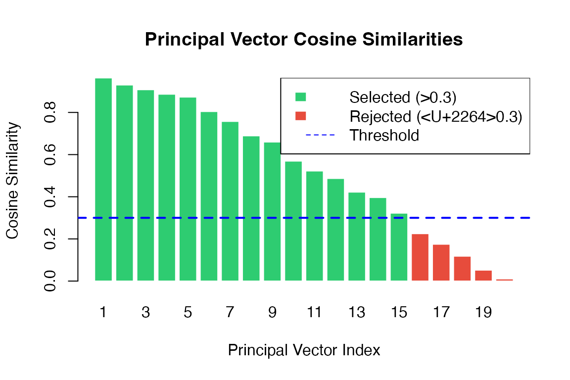

Step 5: Projection

Both datasets are projected onto the aligned subspace defined by the selected principal vectors:

$\mathbf{Z}_s = \mathbf{X}_s \mathbf{S}$ $\mathbf{Z}_t = \mathbf{X}_t \mathbf{S}$

where $\mathbf{S}$ contains the source principal vector loadings.

Step 6: Weighted k-NN Imputation

For each spatial cell $i$ , find $k$ nearest scRNA-seq cells using cosine distance:

$d(a, b) = 1 - \frac{a \cdot b}{\|a\| \|b\|}$

Expression is predicted as a weighted average:

$\hat{y}_i = \sum_{j \in \mathcal{N}_k(i)} w_{ij} \cdot y_j$

where weights are computed as:

$w_{ij} = \frac{1 - d_{ij}/\sum_k d_{ik}}{|\mathcal{N}_k| - 1}$

set.seed(42)

# Demonstrate KNN with cosine distance
query <- matrix(c(1, 0), nrow = 1)
ref <- matrix(c(
  0.9, 0.1,   # Close to query
  0.7, 0.3,   # Medium distance
  0.5, 0.5,   # Farther
  0.1, 0.9    # Far
), nrow = 4, byrow = TRUE)

# Compute KNN
knn_result <- cosine_knn(query, ref, k = 3)

# Visualize
plot(ref[,1], ref[,2], pch = 19, cex = 2,
     xlim = c(-0.2, 1.2), ylim = c(-0.2, 1.2),
     xlab = "Dimension 1", ylab = "Dimension 2",
     main = "Cosine KNN Illustration",
     col = c("#2ecc71", "#f39c12", "#e74c3c", "#95a5a6"))
points(query[1,1], query[1,2], pch = 18, cex = 3, col = "#3498db")

# Draw connections to neighbors
for (i in 1:3) {
  idx <- knn_result$indices[1, i]
  lines(c(query[1,1], ref[idx,1]), c(query[1,2], ref[idx,2]), 
        lty = 2, col = "#3498db", lwd = 1.5)
}

legend("topright", 
       legend = c("Query", "NN 1", "NN 2", "NN 3", "Not selected"),
       pch = c(18, 19, 19, 19, 19),
       col = c("#3498db", "#2ecc71", "#f39c12", "#e74c3c", "#95a5a6"),
       pt.cex = c(2, 1.5, 1.5, 1.5, 1.5))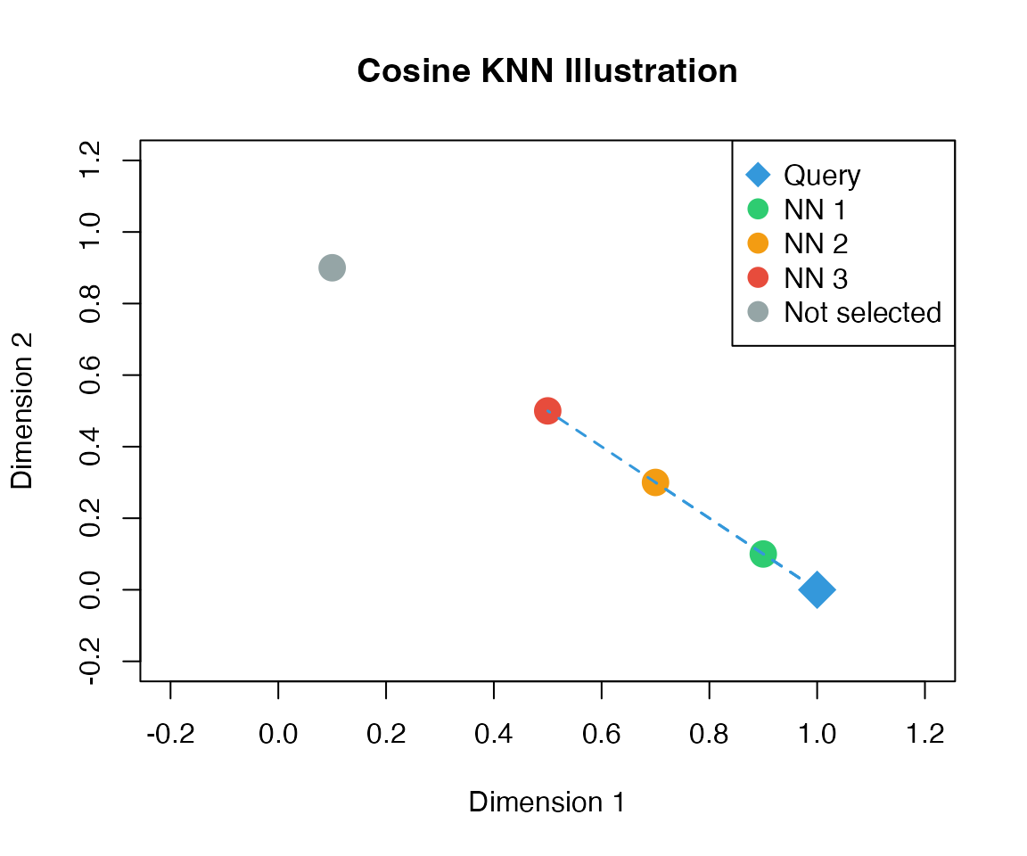


cat("Cosine distances to query:\n")
#> Cosine distances to query:
for (i in 1:4) {
  d <- 1 - sum(query * ref[i,]) / (sqrt(sum(query^2)) * sqrt(sum(ref[i,]^2)))
  cat(sprintf("  Reference %d: %.4f\n", i, d))
}
#>   Reference 1: 0.0061
#>   Reference 2: 0.0809
#>   Reference 3: 0.2929
#>   Reference 4: 0.8896

Comparison with Python Implementation

SpaGER produces numerically equivalent results to the original Python SpaGE:

set.seed(42)

# Z-score comparison
X <- matrix(rnorm(30), nrow = 10, ncol = 3)
X_r <- zscore(X)

# Manual calculation (matching scipy.stats.zscore)
X_manual <- scale(X, center = TRUE, scale = TRUE) * sqrt(nrow(X) / (nrow(X) - 1))

cat("Maximum difference from Python-equivalent calculation:", 
    max(abs(X_r - X_manual)), "\n")
#> Maximum difference from Python-equivalent calculation: 4.440892e-16

Summary

The SpaGE algorithm workflow:

┌─────────────────┐     ┌─────────────────┐
│  Spatial Data   │     │  scRNA-seq Data │
│  (limited genes)│     │ (full genome)   │
└────────┬────────┘     └────────┬────────┘
         │                       │
         ▼                       ▼
    ┌────────────────────────────────┐
    │     Z-score Standardization     │
    └────────────────────────────────┘
         │                       │
         ▼                       ▼
    ┌──────────┐           ┌──────────┐
    │   PCA    │           │   PCA    │
    └────┬─────┘           └────┬─────┘
         │                       │
         └───────────┬───────────┘
                     ▼
    ┌────────────────────────────────┐
    │    Principal Vectors (SVD)     │
    │    Select PVs with sim > 0.3   │
    └────────────────────────────────┘
                     │
                     ▼
    ┌────────────────────────────────┐
    │    Project onto aligned space   │
    └────────────────────────────────┘
                     │
                     ▼
    ┌────────────────────────────────┐
    │   Weighted k-NN Imputation      │
    │   (cosine distance)             │
    └────────────────────────────────┘
                     │
                     ▼
    ┌────────────────────────────────┐
    │    Predicted Gene Expression    │
    └────────────────────────────────┘

References

Abdelaal T, et al. (2020). SpaGE: Spatial Gene Enhancement using scRNA-seq. Nucleic Acids Research, 48(18):e107.
Mourragui S, et al. (2019). PRECISE: A domain adaptation approach to transfer predictors of drug response from pre-clinical models to tumors. Bioinformatics, 35(14):i510-i519.

Session Information

sessionInfo()
#> R version 4.4.0 (2024-04-24)
#> Platform: aarch64-apple-darwin20
#> Running under: macOS 15.6.1
#> 
#> Matrix products: default
#> BLAS:   /Library/Frameworks/R.framework/Versions/4.4-arm64/Resources/lib/libRblas.0.dylib 
#> LAPACK: /Library/Frameworks/R.framework/Versions/4.4-arm64/Resources/lib/libRlapack.dylib;  LAPACK version 3.12.0
#> 
#> locale:
#> [1] C
#> 
#> time zone: Asia/Shanghai
#> tzcode source: internal
#> 
#> attached base packages:
#> [1] stats     graphics  grDevices utils     datasets  methods   base     
#> 
#> other attached packages:
#> [1] SpaGER_1.0.0
#> 
#> loaded via a namespace (and not attached):
#>  [1] cli_3.6.5           knitr_1.51          rlang_1.1.7        
#>  [4] xfun_0.56           otel_0.2.0          textshaping_1.0.4  
#>  [7] jsonlite_2.0.0      future.apply_1.20.1 listenv_0.10.0     
#> [10] htmltools_0.5.9     ragg_1.5.0          sass_0.4.10        
#> [13] rmarkdown_2.30      grid_4.4.0          evaluate_1.0.5     
#> [16] jquerylib_0.1.4     fastmap_1.2.0       yaml_2.3.12        
#> [19] lifecycle_1.0.5     FNN_1.1.4.1         compiler_4.4.0     
#> [22] codetools_0.2-20    irlba_2.3.5.1       fs_1.6.6           
#> [25] Rcpp_1.1.1          htmlwidgets_1.6.4   future_1.69.0      
#> [28] lattice_0.22-7      systemfonts_1.3.1   digest_0.6.39      
#> [31] R6_2.6.1            parallelly_1.46.1   parallel_4.4.0     
#> [34] bslib_0.9.0         Matrix_1.7-4        tools_4.4.0        
#> [37] globals_0.18.0      pkgdown_2.1.3       cachem_1.1.0       
#> [40] desc_1.4.3

Zaoqu Liu

2026-01-25