SpaGER: Visualization and Analysis
Zaoqu Liu
2026-01-25
Source:vignettes/visualization.Rmd
visualization.RmdIntroduction
This vignette demonstrates visualization techniques for SpaGER predictions and analyses, helping you interpret and present your results effectively.
Simulated Dataset
We create a more realistic simulated dataset with biological structure:
# Parameters
n_rna <- 500
n_spatial <- 200
n_shared <- 80
n_predict <- 40

# Create cell type structure (3 cell types)
cell_types <- rep(1:3, length.out = n_rna)
type_means <- c(3, 5, 7)

# scRNA-seq with cell type-specific expression
rna_base <- matrix(0, nrow = n_rna, ncol = n_shared + n_predict)
for (i in 1:n_rna) {
  rna_base[i, ] <- rnorm(n_shared + n_predict, mean = type_means[cell_types[i]], sd = 1)
}
rna_base <- abs(rna_base)
colnames(rna_base) <- c(paste0("Shared", 1:n_shared), paste0("Novel", 1:n_predict))

# Spatial data - mixture of cell types
spatial_types <- sample(1:3, n_spatial, replace = TRUE, prob = c(0.5, 0.3, 0.2))
spatial_base <- matrix(0, nrow = n_spatial, ncol = n_shared)
for (i in 1:n_spatial) {
  spatial_base[i, ] <- rnorm(n_shared, mean = type_means[spatial_types[i]], sd = 1.2)
}
spatial_base <- abs(spatial_base)
colnames(spatial_base) <- paste0("Shared", 1:n_shared)

# Add spatial coordinates
coords <- data.frame(
  x = runif(n_spatial, 0, 100),
  y = runif(n_spatial, 0, 100)
)
rownames(coords) <- paste0("Spot", 1:n_spatial)
rownames(spatial_base) <- rownames(coords)

cat("Data created:\n")
#> Data created:
cat("  scRNA-seq:", n_rna, "cells,", ncol(rna_base), "genes\n")
#>   scRNA-seq: 500 cells, 120 genes
cat("  Spatial:", n_spatial, "spots,", ncol(spatial_base), "genes\n")
#>   Spatial: 200 spots, 80 genes
Run SpaGE Prediction
predicted <- SpaGE(
  spatial_data = as.data.frame(spatial_base),
  rna_data = as.data.frame(rna_base),
  n_pv = 30,
  n_neighbors = 50,
  verbose = FALSE
)

cat("Predicted", ncol(predicted), "novel genes\n")
#> Predicted 40 novel genes
Visualizing Principal Vector Selection
# Get PV information
similarities <- attr(predicted, "similarities")
n_pv_used <- attr(predicted, "n_pv_used")

par(mfrow = c(1, 2))

# Bar plot of similarities
cols <- ifelse(seq_along(similarities) <= n_pv_used, "#3498db", "#bdc3c7")
barplot(similarities,
        names.arg = seq_along(similarities),
        col = cols,
        border = "white",
        main = "Principal Vector Selection",
        xlab = "PV Index",
        ylab = "Cosine Similarity",
        ylim = c(0, 1))
abline(h = 0.3, col = "#e74c3c", lty = 2, lwd = 2)
legend("topright",
       legend = c("Selected", "Rejected", "Threshold (0.3)"),
       fill = c("#3498db", "#bdc3c7", NA),
       border = c("white", "white", NA),
       lty = c(NA, NA, 2),
       col = c(NA, NA, "#e74c3c"))

# Cumulative variance
cum_var <- cumsum(similarities^2) / sum(similarities^2)
plot(cum_var, type = "b", pch = 19, col = "#2ecc71",
     main = "Cumulative Variance Captured",
     xlab = "Number of PVs",
     ylab = "Cumulative Proportion",
     xlim = c(1, length(similarities)))
abline(v = n_pv_used, col = "#e74c3c", lty = 2)
abline(h = cum_var[n_pv_used], col = "#e74c3c", lty = 2)
text(n_pv_used + 1, cum_var[n_pv_used],
     sprintf("%.1f%%", cum_var[n_pv_used] * 100), pos = 4)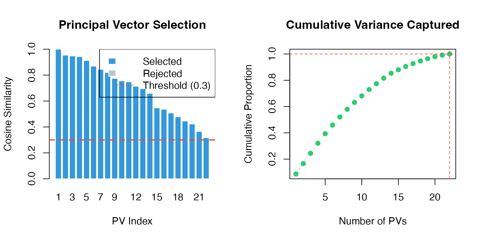
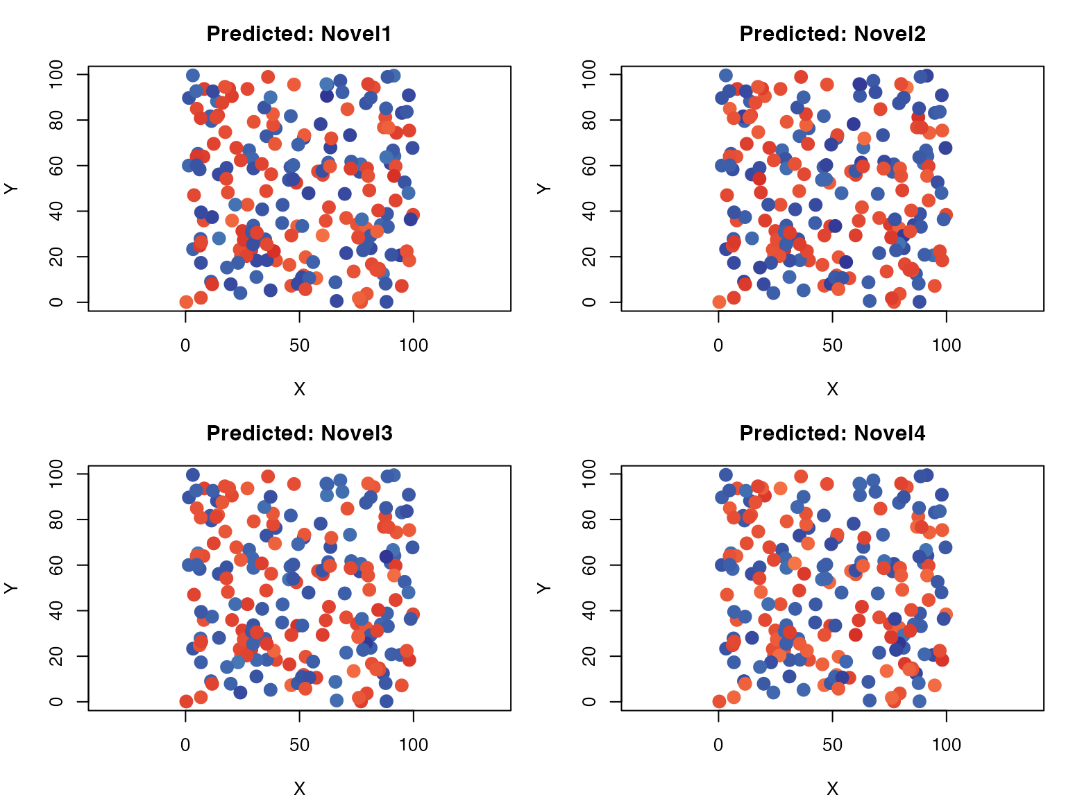
Spatial Expression Patterns
# Function to plot spatial expression
plot_spatial <- function(coords, values, title, col_palette = NULL) {
  if (is.null(col_palette)) {
    col_palette <- colorRampPalette(c("#313695", "#4575b4", "#74add1",
                                       "#abd9e9", "#ffffbf", "#fee090",
                                       "#fdae61", "#f46d43", "#d73027"))(100)
  }

  # Normalize values to [0, 1]
  val_norm <- (values - min(values)) / (max(values) - min(values) + 1e-10)
  cols <- col_palette[ceiling(val_norm * 99) + 1]

  plot(coords$x, coords$y, pch = 19, cex = 1.5,
       col = cols, xlab = "X", ylab = "Y", main = title,
       asp = 1)
}

# Plot predicted genes
par(mfrow = c(2, 2), mar = c(4, 4, 3, 1))

for (i in 1:4) {
  gene <- colnames(predicted)[i]
  plot_spatial(coords, predicted[, gene], paste("Predicted:", gene))
}
Cross-Validation Results
# Run CV
cv_results <- SpaGE_cv(
  spatial_data = as.data.frame(spatial_base),
  rna_data = as.data.frame(rna_base[, paste0("Shared", 1:n_shared)]),
  n_pv = 20,
  genes = paste0("Shared", 1:20),
  verbose = FALSE
)

par(mfrow = c(1, 2))

# Histogram
hist(cv_results$correlation, breaks = 15, col = "#3498db", border = "white",
     main = "Cross-Validation Performance",
     xlab = "Spearman Correlation",
     xlim = c(-0.2, 1))
abline(v = median(cv_results$correlation), col = "#e74c3c", lwd = 2, lty = 2)
abline(v = mean(cv_results$correlation), col = "#2ecc71", lwd = 2, lty = 2)
legend("topleft",
       legend = c(paste("Median:", round(median(cv_results$correlation), 3)),
                  paste("Mean:", round(mean(cv_results$correlation), 3))),
       col = c("#e74c3c", "#2ecc71"), lty = 2, lwd = 2)

# Per-gene plot
cv_ordered <- cv_results[order(cv_results$correlation, decreasing = TRUE), ]
barplot(cv_ordered$correlation,
        names.arg = substr(cv_ordered$gene, 7, 10),
        las = 2,
        col = ifelse(cv_ordered$correlation > 0.3, "#2ecc71", "#e74c3c"),
        border = "white",
        main = "Per-Gene Correlation",
        ylab = "Spearman Correlation")
abline(h = 0.3, lty = 2)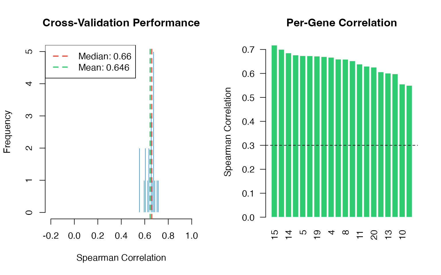
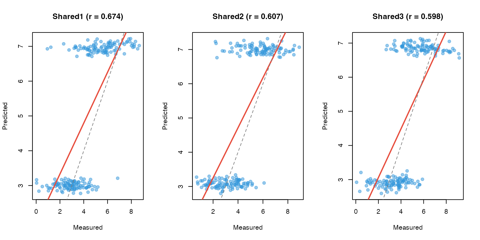
Measured vs Predicted Scatter Plots
# For CV genes, compare measured vs predicted
par(mfrow = c(1, 3))

for (i in 1:3) {
  gene <- cv_results$gene[i]

  # Get measured values
  measured <- spatial_base[, gene]

  # Run prediction for this gene
  spatial_minus <- spatial_base[, setdiff(colnames(spatial_base), gene)]
  pred_single <- SpaGE(
    spatial_data = as.data.frame(spatial_minus),
    rna_data = as.data.frame(rna_base[, paste0("Shared", 1:n_shared)]),
    n_pv = 20,
    genes_to_predict = gene,
    verbose = FALSE
  )

  predicted_vals <- pred_single[, gene]
  cor_val <- cor(measured, predicted_vals, method = "spearman")

  plot(measured, predicted_vals, pch = 19, col = adjustcolor("#3498db", 0.5),
       xlab = "Measured", ylab = "Predicted",
       main = sprintf("%s (r = %.3f)", gene, cor_val))
  abline(lm(predicted_vals ~ measured), col = "#e74c3c", lwd = 2)

  # Add identity line
  abline(0, 1, lty = 2, col = "gray50")
}
Expression Distribution Comparison
par(mfrow = c(1, 2))

# Density plot for predicted genes
gene1 <- colnames(predicted)[1]
gene2 <- colnames(predicted)[2]

# Use density estimation
d1 <- density(predicted[, gene1])
d2 <- density(predicted[, gene2])

plot(d1, col = "#3498db", lwd = 2,
     main = "Predicted Expression Distribution",
     xlab = "Expression Level",
     xlim = range(c(d1$x, d2$x)),
     ylim = range(c(d1$y, d2$y)))
lines(d2, col = "#e74c3c", lwd = 2)
legend("topright", legend = c(gene1, gene2),
       col = c("#3498db", "#e74c3c"), lwd = 2)

# Box plot
boxplot(predicted[, 1:10],
        col = "#3498db",
        border = "#2c3e50",
        main = "Predicted Expression (First 10 Genes)",
        xlab = "Gene",
        ylab = "Expression",
        las = 2,
        names = substr(colnames(predicted)[1:10], 1, 8))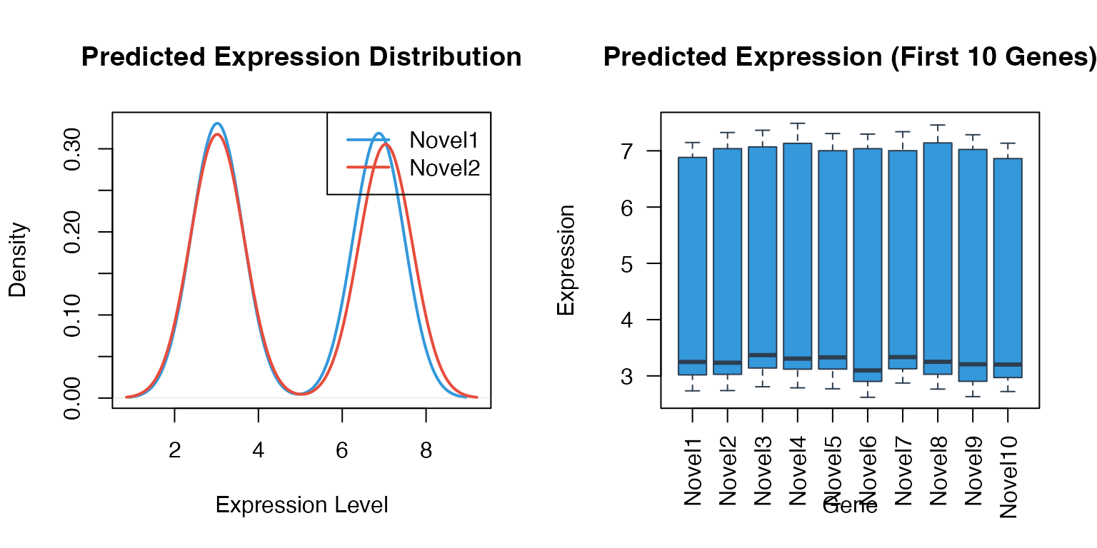
Correlation Heatmap
# Compute correlation matrix for predicted genes
pred_subset <- predicted[, 1:15]
cor_mat <- cor(pred_subset, method = "spearman")

# Simple heatmap
heatmap(cor_mat,
        col = colorRampPalette(c("#3498db", "white", "#e74c3c"))(50),
        scale = "none",
        main = "Gene-Gene Correlation (Predicted)",
        margins = c(8, 8))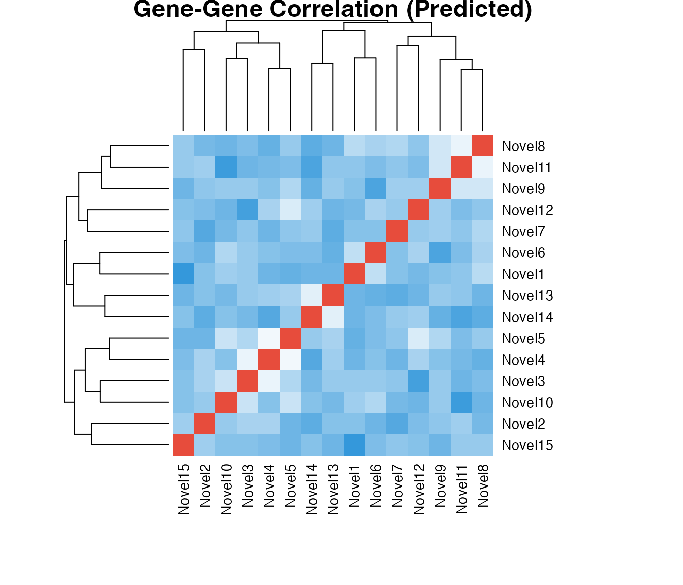
Summary Statistics
cat("=== SpaGE Prediction Summary ===\n\n")
#> === SpaGE Prediction Summary ===

cat("Input Data:\n")
#> Input Data:
cat(sprintf("  Spatial spots: %d\n", nrow(spatial_base)))
#>   Spatial spots: 200
cat(sprintf("  scRNA-seq cells: %d\n", nrow(rna_base)))
#>   scRNA-seq cells: 500
cat(sprintf("  Shared genes: %d\n", n_shared))
#>   Shared genes: 80
cat(sprintf("  Novel genes predicted: %d\n", ncol(predicted)))
#>   Novel genes predicted: 40

cat("\nPrincipal Vectors:\n")
#>
#> Principal Vectors:
cat(sprintf("  Requested: %d\n", attr(predicted, "n_pv")))
#>   Requested: 30
cat(sprintf("  Used (sim > 0.3): %d\n", attr(predicted, "n_pv_used")))
#>   Used (sim > 0.3): 22
cat(sprintf("  Mean similarity: %.3f\n", mean(attr(predicted, "similarities"))))
#>   Mean similarity: 0.694

cat("\nCross-Validation:\n")
#>
#> Cross-Validation:
cat(sprintf("  Genes tested: %d\n", nrow(cv_results)))
#>   Genes tested: 20
cat(sprintf("  Mean correlation: %.3f\n", mean(cv_results$correlation)))
#>   Mean correlation: 0.646
cat(sprintf("  Median correlation: %.3f\n", median(cv_results$correlation)))
#>   Median correlation: 0.660
cat(sprintf("  Genes with r > 0.3: %d (%.1f%%)\n",
            sum(cv_results$correlation > 0.3),
            100 * mean(cv_results$correlation > 0.3)))
#>   Genes with r > 0.3: 20 (100.0%)

cat("\nPredicted Expression:\n")
#>
#> Predicted Expression:
cat(sprintf("  Mean: %.3f\n", mean(as.matrix(predicted))))
#>   Mean: 4.962
cat(sprintf("  SD: %.3f\n", sd(as.matrix(predicted))))
#>   SD: 1.997
cat(sprintf("  Range: [%.3f, %.3f]\n", min(predicted), max(predicted)))
#>   Range: [2.564, 7.563]
Exporting Results
# Export predicted expression
write.csv(predicted, "spage_predictions.csv")

# Export CV results
write.csv(cv_results, "spage_cv_results.csv")

# Export for visualization in other tools
saveRDS(list(
  predictions = predicted,
  coordinates = coords,
  cv_results = cv_results,
  metadata = list(
    n_pv = attr(predicted, "n_pv"),
    n_pv_used = attr(predicted, "n_pv_used"),
    similarities = attr(predicted, "similarities")
  )
), "spage_results.rds")
Session Information
sessionInfo()
#> R version 4.4.0 (2024-04-24)
#> Platform: aarch64-apple-darwin20
#> Running under: macOS 15.6.1
#>
#> Matrix products: default
#> BLAS:   /Library/Frameworks/R.framework/Versions/4.4-arm64/Resources/lib/libRblas.0.dylib
#> LAPACK: /Library/Frameworks/R.framework/Versions/4.4-arm64/Resources/lib/libRlapack.dylib;  LAPACK version 3.12.0
#>
#> locale:
#> [1] C
#>
#> time zone: Asia/Shanghai
#> tzcode source: internal
#>
#> attached base packages:
#> [1] stats     graphics  grDevices utils     datasets  methods   base
#>
#> other attached packages:
#> [1] SpaGER_1.0.0
#>
#> loaded via a namespace (and not attached):
#>  [1] cli_3.6.5           knitr_1.51          rlang_1.1.7
#>  [4] xfun_0.56           otel_0.2.0          textshaping_1.0.4
#>  [7] jsonlite_2.0.0      future.apply_1.20.1 listenv_0.10.0
#> [10] htmltools_0.5.9     ragg_1.5.0          sass_0.4.10
#> [13] rmarkdown_2.30      grid_4.4.0          evaluate_1.0.5
#> [16] jquerylib_0.1.4     fastmap_1.2.0       yaml_2.3.12
#> [19] lifecycle_1.0.5     FNN_1.1.4.1         compiler_4.4.0
#> [22] codetools_0.2-20    irlba_2.3.5.1       fs_1.6.6
#> [25] Rcpp_1.1.1          htmlwidgets_1.6.4   future_1.69.0
#> [28] lattice_0.22-7      systemfonts_1.3.1   digest_0.6.39
#> [31] R6_2.6.1            parallelly_1.46.1   parallel_4.4.0
#> [34] bslib_0.9.0         Matrix_1.7-4        tools_4.4.0
#> [37] globals_0.18.0      pkgdown_2.1.3       cachem_1.1.0
#> [40] desc_1.4.3