Algorithm and Methodology

Zaoqu Liu

2026-01-23

Theoretical Background

Copy Number Variations in Cancer

Copy Number Variations (CNVs) are structural alterations in the genome where segments of DNA are duplicated (amplifications) or deleted (losses). In cancer:

• Amplifications often harbor oncogenes (e.g., MYC, ERBB2)
• Deletions frequently affect tumor suppressor genes (e.g., TP53, CDKN2A)
• CNV patterns define tumor subclones with distinct evolutionary trajectories

Expression-Based CNV Inference

The central premise of expression-based CNV detection is:

$$\text{Gene Expression} \propto \text{Gene Copy Number}$$

Genes in amplified regions tend to show elevated expression, while genes in deleted regions show reduced expression. By analyzing expression patterns across genomically ordered genes, we can infer underlying CNVs.

Algorithm Pipeline

The fastCNV algorithm consists of six main steps:

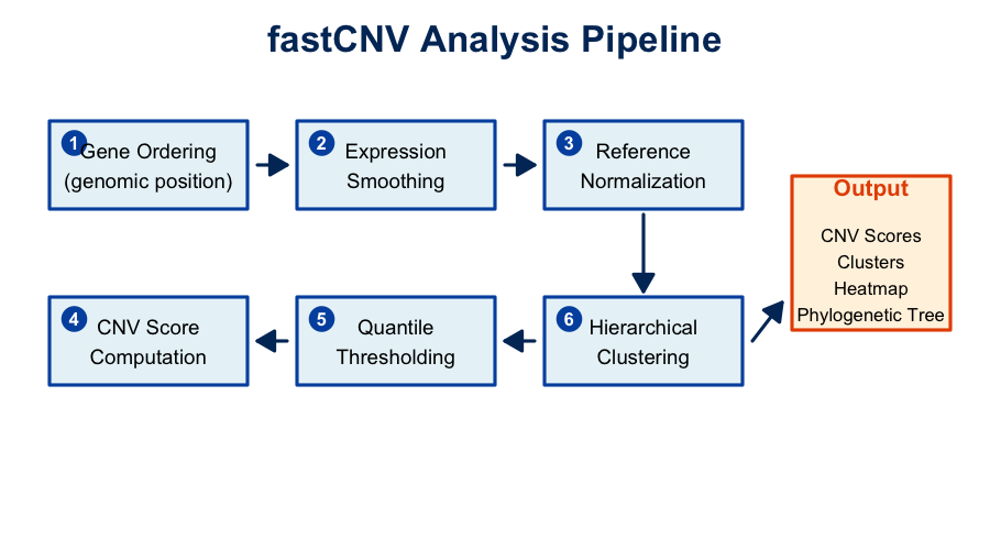
Overview of the fastCNV analysis pipeline.

Pipeline Steps:

1. Gene Ordering: Sort genes by chromosome and genomic position
2. Expression Smoothing: Apply sliding window across ordered genes
3. Reference Normalization: Center scores using reference (normal) cells
4. Score Computation: Calculate CNV scores per window
5. Thresholding: Apply quantile-based noise filtering
6. Clustering: Identify CNV-based subpopulations

Step 1: Gene Ordering

Genes are ordered by their genomic coordinates:

1. Chromosome ordering: 1, 2, …, 22, X
2. Position ordering: By transcription start site (TSS)

# Gene metadata contains genomic coordinates
data("geneMetadata", package = "fastCNV")
head(geneMetadata)

This ordering ensures that adjacent genes in our analysis are also adjacent in the genome.

Step 2: Sliding Window Smoothing

Raw gene expression is noisy. We apply a sliding window approach:

$$S_w = \frac{1}{|W|} \sum_{g \in W} E_g$$

Where: - $S_w$ = smoothed score for window $w$ - $W$ = set of genes in the window - $E_g$ = normalized expression of gene $g$ - $|W|$ = window size (default: 150 genes)

Why smoothing?

• Reduces single-gene noise
• Captures regional expression patterns
• Mimics the resolution of array-based CNV detection

# Window size affects resolution vs. noise trade-off
# Smaller windows → higher resolution, more noise
# Larger windows → smoother profiles, lower resolution

result <- fastCNV(
  seuratObj = seurat_obj,
  sampleName = "Sample1",
  referenceVar = "cell_type",
  referenceLabel = c("Normal"),
  windowSize = 150  # Default: 150 genes per window
)

Step 3: Reference Normalization

The key innovation in expression-based CNV detection is reference normalization:

$$CNV_{cell} = S_{cell} - \bar{S}_{reference}$$

Reference cells (typically non-malignant cells like fibroblasts, immune cells) provide the baseline expression expected without CNVs.

Important considerations:

• Reference cells should be diploid (normal copy number)
• Multiple reference cell types improve robustness
• For tumors, use adjacent normal tissue or known normal populations

# Good reference cell types:
# - Fibroblasts
# - Endothelial cells
# - Immune cells (T cells, B cells, macrophages)
# - Normal epithelial cells (if available)

result <- fastCNV(
  seuratObj = seurat_obj,
  sampleName = "Sample1",
  referenceVar = "cell_type",
  referenceLabel = c("Fibroblast", "T_cell", "Endothelial")
)

Step 4: Score Computation

For each cell and each genomic window, we compute:

$$CNV\_score_{c,w} = \bar{E}_{c,w} - \bar{E}_{ref,w}$$

Where: - $\bar{E}_{c,w}$ = mean expression of cell $c$ in window $w$ - $\bar{E}_{ref,w}$ = mean expression of reference cells in window $w$

Interpretation: - Positive scores → potential amplification - Negative scores → potential deletion - Near-zero scores → normal copy number

Step 5: Quantile-Based Thresholding

To reduce false positives from biological noise:

1. Compute quantiles (default: 1st and 99th percentiles)
2. Scores within quantile range → set to 0 (no CNV)
3. Extreme scores → retained as putative CNVs

# thresholdPercentile controls stringency
# Higher values → more stringent (fewer CNV calls)
# Lower values → more sensitive (more CNV calls)

result <- fastCNV(
  seuratObj = seurat_obj,
  sampleName = "Sample1",
  referenceVar = "cell_type",
  referenceLabel = c("Normal"),
  thresholdPercentile = 0.01  # Default: 1st/99th percentile
)

Step 6: Hierarchical Clustering

Cells are clustered based on their CNV profiles:

1. Compute pairwise distances between CNV profiles
2. Build hierarchical clustering tree
3. Cut tree to define subclones

# Automatic clustering
result <- CNVCluster(
  seuratObj = result,
  referenceVar = "cell_type",
  tumorLabel = "Tumor",
  k = NULL,  # Auto-determine number of clusters
  plotDendrogram = TRUE,
  plotElbowPlot = TRUE
)

# Manual specification
result <- CNVCluster(
  seuratObj = result,
  referenceVar = "cell_type",
  tumorLabel = "Tumor",
  k = 4  # Force 4 clusters
)

Mathematical Details

Distance Metric

The default distance metric is correlation distance:

$$d(x, y) = 1 - \frac{\sum(x_i - \bar{x})(y_i - \bar{y})}{\sqrt{\sum(x_i - \bar{x})^2 \sum(y_i - \bar{y})^2}}$$

This metric is robust to: - Differences in overall expression level - Technical batch effects

CNV Classification

Final CNV calls are classified as:

Classification	Criteria
Amplification	Score > threshold
Deletion	Score < -threshold
Neutral	-threshold ≤ Score ≤ threshold

# Classify CNV calls
result <- CNVClassification(
  seuratObj = result,
  referenceVar = "cell_type",
  referenceLabel = c("Normal")
)

Performance Optimization

Vectorized Operations

fastCNV 2.0 uses vectorized operations for efficiency:

# Old approach (slow)
# for (i in 1:n) { result[i] <- compute(data[i]) }

# New approach (fast)
# result <- vectorized_compute(data)

Memory Management

For large datasets, fastCNV implements strategic garbage collection:

# Automatic memory cleanup
result <- fastCNV(
  seuratObj = large_seurat,
  sampleName = "Large_sample",
  referenceVar = "cell_type",
  referenceLabel = c("Normal")
)
# gc() is called at key checkpoints

Algorithm Parameters Summary

Parameter	Description	Default	Impact
windowSize	Genes per window	150	Resolution vs. noise
topNGenes	Genes to analyze	7000	Coverage vs. speed
thresholdPercentile	Noise filter	0.01	Sensitivity vs. specificity
aggregFactor	Spatial binning	10	Coverage vs. resolution

Validation and Quality Control

Checking Results

# 1. Verify reference cells are diploid
# Reference cells should show minimal CNV signal
ref_cells <- which(result$cell_type %in% c("Normal"))
mean_ref_signal <- mean(abs(result@assays$CNVScores[, ref_cells]))
message("Mean reference CNV signal: ", round(mean_ref_signal, 4))

# 2. Check known CNV regions
# If you know expected CNVs, verify they are detected
# e.g., chromosome 7 gain in glioblastoma

# 3. Compare with DNA-based CNV calls (if available)

References

1. Patel AP, et al. (2014). Single-cell RNA-seq highlights intratumoral heterogeneity in primary glioblastoma. Science.

2. Tirosh I, et al. (2016). Dissecting the multicellular ecosystem of metastatic melanoma by single-cell RNA-seq. Science.

3. Fan J, et al. (2018). Linking transcriptional and genetic tumor heterogeneity through allele analysis of single-cell RNA-seq data. Genome Research.

Session Info

sessionInfo()
#> R version 4.4.0 (2024-04-24)
#> Platform: aarch64-apple-darwin20
#> Running under: macOS 15.6.1
#> 
#> Matrix products: default
#> BLAS:   /Library/Frameworks/R.framework/Versions/4.4-arm64/Resources/lib/libRblas.0.dylib 
#> LAPACK: /Library/Frameworks/R.framework/Versions/4.4-arm64/Resources/lib/libRlapack.dylib;  LAPACK version 3.12.0
#> 
#> locale:
#> [1] C
#> 
#> time zone: Asia/Shanghai
#> tzcode source: internal
#> 
#> attached base packages:
#> [1] stats     graphics  grDevices utils     datasets  methods   base     
#> 
#> loaded via a namespace (and not attached):
#>  [1] digest_0.6.39     desc_1.4.3        R6_2.6.1          fastmap_1.2.0    
#>  [5] xfun_0.56         cachem_1.1.0      knitr_1.51        htmltools_0.5.9  
#>  [9] rmarkdown_2.30    lifecycle_1.0.5   cli_3.6.5         sass_0.4.10      
#> [13] pkgdown_2.1.3     textshaping_1.0.4 jquerylib_0.1.4   systemfonts_1.3.1
#> [17] compiler_4.4.0    tools_4.4.0       ragg_1.5.0        bslib_0.9.0      
#> [21] evaluate_1.0.5    yaml_2.3.12       otel_0.2.0        jsonlite_2.0.0   
#> [25] rlang_1.1.7       fs_1.6.6          htmlwidgets_1.6.4