Overview
fastCNV provides comprehensive visualization tools for CNV analysis results. This vignette covers:
- CNV Heatmaps - Genome-wide CNV profiles
- Phylogenetic Trees - Clonal evolution visualization
- Chromosome Arm Plots - Arm-level CNV summary
- Spatial CNV Maps - CNV patterns in tissue context
CNV Heatmaps
Example CNV Heatmap
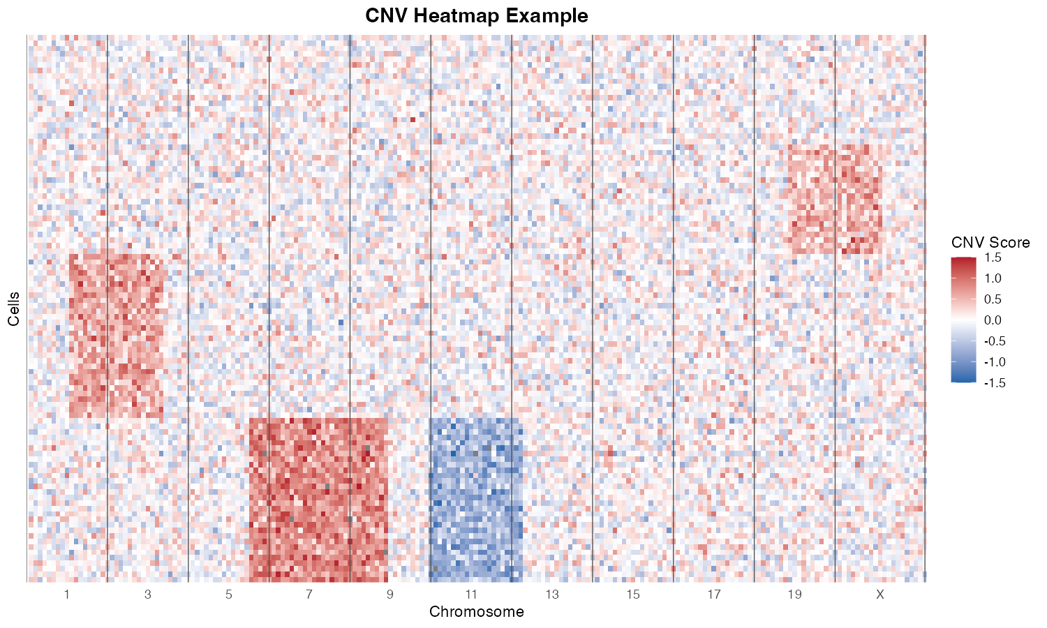
CNV heatmap showing chromosomal alterations. Rows represent cells, columns represent genomic windows. Blue = deletion, Red = amplification.
Basic Heatmap
The plotCNVResults() function generates
publication-ready heatmaps:
library(fastCNV)

# Generate CNV heatmap
plotCNVResults(
  seuratObj = result,
  referenceVar = "cell_type",
  tumorLabel = "Tumor"
)
Customizing Heatmaps
Split by Cell Type
plotCNVResults(
  seuratObj = result,
  referenceVar = "cell_type",
  tumorLabel = "Tumor",
  splitPlotOnVar = "cell_subtype"  # Split rows by subtype
)
Split by CNV Clusters
plotCNVResults(
  seuratObj = result,
  referenceVar = "cell_type",
  tumorLabel = "Tumor",
  splitPlotOnVar = "cnv_clusters"  # Group by CNV clusters
)
Custom Color Scheme
The heatmap uses a diverging color scale: - Blue: Deletions (negative CNV scores) - White: Neutral (no alteration) - Red: Amplifications (positive CNV scores)
# The default color scheme is optimized for CNV visualization
# Colors are scaled to the data range with balanced mapping
Heatmap Components
A typical CNV heatmap includes:
┌─────────────────────────────────────────────────────────────┐
│                    Chromosome Labels (1-22, X)              │
├─────────────────────────────────────────────────────────────┤
│  Row      │                                                 │
│  Anno-    │          CNV Score Matrix                       │
│  tations  │          (cells × genomic windows)              │
│           │                                                 │
│  - Cell   │  Blue = Deletion                                │
│    type   │  White = Neutral                                │
│  - Clone  │  Red = Amplification                            │
│           │                                                 │
├─────────────────────────────────────────────────────────────┤
│                    Color Legend                             │
└─────────────────────────────────────────────────────────────┘
Phylogenetic Trees
Example Dendrogram
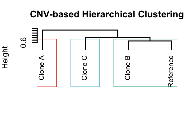
Hierarchical clustering dendrogram based on CNV profiles, showing the relationship between different clones.
Building CNV Trees
CNV profiles can be used to reconstruct clonal phylogenies:
# Build phylogenetic tree from CNV clusters
tree <- CNVTree(
  seuratObj = result,
  referenceVar = "cell_type",
  tumorLabel = "Tumor",
  cnv_thresh = 0.15
)
Visualizing Trees
# Plot the phylogenetic tree
plotCNVTree(
  tree = tree,
  seuratObj = result,
  referenceVar = "cell_type",
  tumorLabel = "Tumor"
)
Annotated Trees
Add CNV event annotations to tree branches:
# Annotate tree with CNV events
annotated_tree <- annotateCNVTree(
  tree = tree,
  seuratObj = result,
  cnv_thresh = 0.15
)

# Plot with annotations
plotCNVTree(
  tree = annotated_tree,
  seuratObj = result,
  referenceVar = "cell_type",
  tumorLabel = "Tumor",
  show_annotations = TRUE
)Chromosome Arm-Level Analysis
Example: CNV Fraction per Chromosome Arm
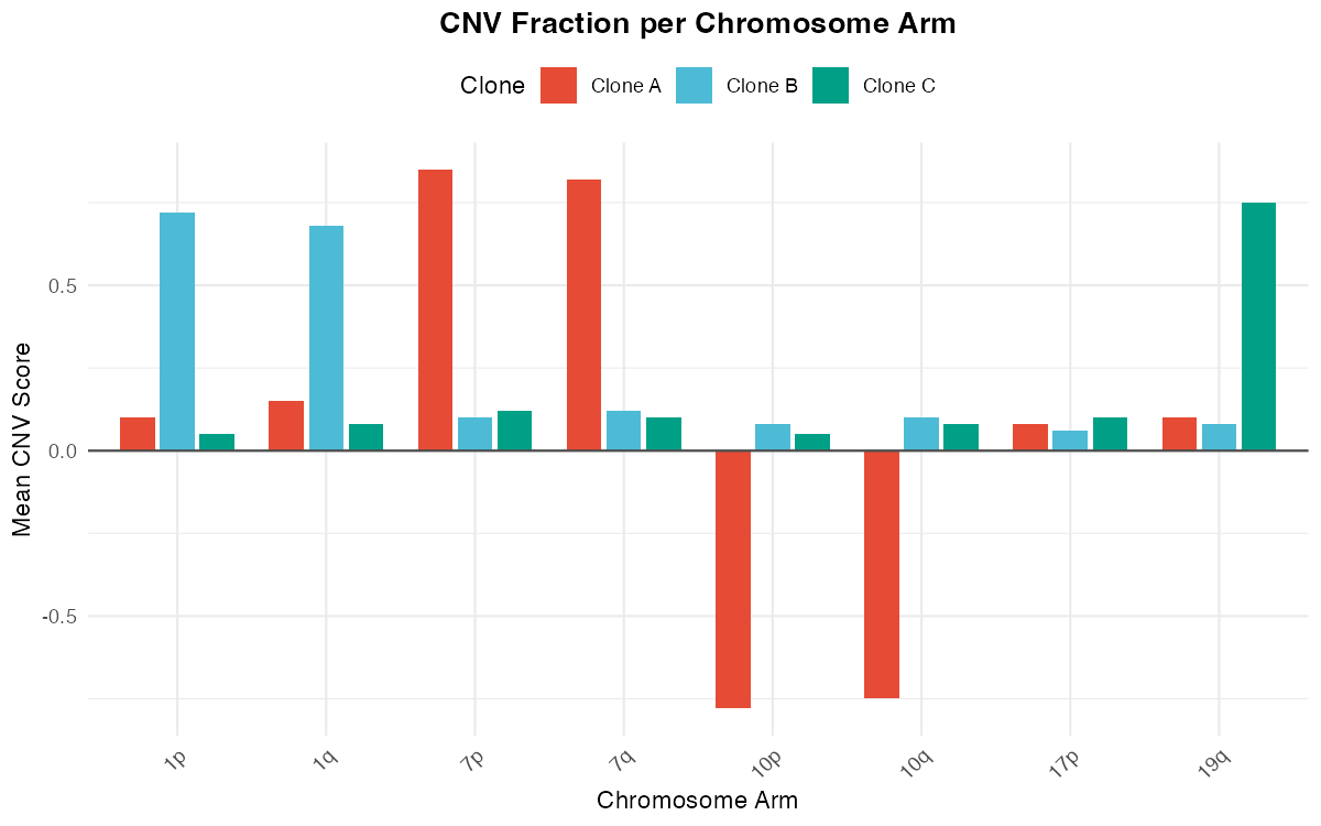
Bar plot showing mean CNV scores per chromosome arm for different clones.
Computing Arm-Level CNVs
# Calculate CNV fraction per chromosome arm
result <- CNVPerChromosomeArm(
  seuratObj = result,
  referenceVar = "cell_type",
  tumorLabel = "Tumor"
)

# View arm-level data
head(result$cnv_per_arm)
Visualizing Arm-Level CNVs
library(ggplot2)

# Extract arm-level data
arm_data <- result$cnv_per_arm

# Create bar plot
ggplot(arm_data, aes(x = arm, y = cnv_fraction, fill = cnv_type)) +
  geom_bar(stat = "identity") +
  facet_wrap(~cluster, ncol = 1) +
  theme_minimal() +
  theme(axis.text.x = element_text(angle = 45, hjust = 1)) +
  labs(
    title = "CNV Fraction per Chromosome Arm",
    x = "Chromosome Arm",
    y = "Fraction of Cells with CNV"
  )
Spatial CNV Visualization
Visium Data
library(Seurat)

# Plot CNV clusters on tissue
SpatialDimPlot(
  result,
  group.by = "cnv_clusters",
  pt.size.factor = 1.6
)
Visium HD Data
# For Visium HD, use the specialized function
plotCNVResultsHD(
  seuratObj = result,
  referenceVar = "region",
  tumorLabel = "Tumor"
)
Combining Spatial and CNV Information
# Create a multi-panel figure
library(patchwork)

# Panel 1: Cell type annotation
p1 <- SpatialDimPlot(result, group.by = "cell_type")

# Panel 2: CNV clusters
p2 <- SpatialDimPlot(result, group.by = "cnv_clusters")

# Panel 3: CNV score for specific chromosome
p3 <- SpatialFeaturePlot(result, features = "chr7_cnv_score")

# Combine
p1 | p2 | p3
Custom Visualizations
Creating Custom Plots
library(ggplot2)
library(tidyr)

# Example: Plot CNV profile for a single cell
cell_profile <- cnv_scores[, "cell_1"]
window_positions <- 1:length(cell_profile)

ggplot(data.frame(pos = window_positions, cnv = cell_profile)) +

  geom_line(aes(x = pos, y = cnv), color = "steelblue") +
  geom_hline(yintercept = 0, linetype = "dashed", color = "gray50") +
  theme_minimal() +
  labs(
    title = "CNV Profile: Cell 1",
    x = "Genomic Position (window)",
    y = "CNV Score"
  )
Comparing Clusters
# Compare average CNV profiles between clusters
library(dplyr)

# Calculate mean CNV per cluster
cluster_means <- result@meta.data %>%
  group_by(cnv_clusters) %>%
  summarise(
    mean_cnv_fraction = mean(cnv_fraction),
    n_cells = n()
  )

# Plot
ggplot(cluster_means, aes(x = cnv_clusters, y = mean_cnv_fraction, fill = cnv_clusters)) +
  geom_bar(stat = "identity") +
  theme_minimal() +
  labs(
    title = "Mean CNV Fraction by Cluster",
    x = "CNV Cluster",
    y = "Mean CNV Fraction"
  )
Publication-Ready Figures
High-Resolution Export
# Save heatmap as PDF
pdf("cnv_heatmap.pdf", width = 12, height = 8)
plotCNVResults(
  seuratObj = result,
  referenceVar = "cell_type",
  tumorLabel = "Tumor"
)
dev.off()

# Save tree as PDF
pdf("cnv_tree.pdf", width = 8, height = 6)
plotCNVTree(
  tree = tree,
  seuratObj = result,
  referenceVar = "cell_type",
  tumorLabel = "Tumor"
)
dev.off()
Figure Panel Assembly
library(patchwork)
library(ggplot2)

# Create individual panels
p_umap <- DimPlot(result, group.by = "cnv_clusters")
p_spatial <- SpatialDimPlot(result, group.by = "cnv_clusters")

# Assemble figure
figure <- (p_umap | p_spatial) /
          plot_spacer() +
          plot_layout(heights = c(2, 1))

# Save
ggsave("figure_panel.pdf", figure, width = 14, height = 10)
Color Palettes
Default Palettes
fastCNV uses carefully selected color palettes:
# CNV score colors (diverging)
# Blue (-) → White (0) → Red (+)

# Cluster colors (qualitative)
# Uses paletteer for distinct, colorblind-friendly colors
library(paletteer)
cluster_colors <- paletteer_d("ggsci::default_nejm")Tips and Best Practices
1. Heatmap Ordering
- Order cells by cluster, then by similarity within cluster
- Use dendrograms to show hierarchical relationships
2. Color Scaling
- Center the color scale at zero
- Use symmetric limits for amplifications and deletions
Session Info
sessionInfo()
#> R version 4.4.0 (2024-04-24)
#> Platform: aarch64-apple-darwin20
#> Running under: macOS 15.6.1
#>
#> Matrix products: default
#> BLAS:   /Library/Frameworks/R.framework/Versions/4.4-arm64/Resources/lib/libRblas.0.dylib
#> LAPACK: /Library/Frameworks/R.framework/Versions/4.4-arm64/Resources/lib/libRlapack.dylib;  LAPACK version 3.12.0
#>
#> locale:
#> [1] C
#>
#> time zone: Asia/Shanghai
#> tzcode source: internal
#>
#> attached base packages:
#> [1] stats     graphics  grDevices utils     datasets  methods   base
#>
#> loaded via a namespace (and not attached):
#>  [1] digest_0.6.39     desc_1.4.3        R6_2.6.1          fastmap_1.2.0
#>  [5] xfun_0.56         cachem_1.1.0      knitr_1.51        htmltools_0.5.9
#>  [9] rmarkdown_2.30    lifecycle_1.0.5   cli_3.6.5         sass_0.4.10
#> [13] pkgdown_2.1.3     textshaping_1.0.4 jquerylib_0.1.4   systemfonts_1.3.1
#> [17] compiler_4.4.0    tools_4.4.0       ragg_1.5.0        bslib_0.9.0
#> [21] evaluate_1.0.5    yaml_2.3.12       otel_0.2.0        jsonlite_2.0.0
#> [25] rlang_1.1.7       fs_1.6.6          htmlwidgets_1.6.4