Introduction
iTALK provides three visualization functions for exploring cell-cell communication:
| Function | Type | Best For |
|---|---|---|
LRPlot() |
Circos plot | Detailed L-R pair visualization |
NetView() |
Network graph | Overall communication topology |
TimePlot() |
Time series | Dynamic changes across conditions |
This vignette demonstrates customization options for each visualization.
Setup
library(iTALK)
library(dplyr)

# Create example L-R pairs data
set.seed(42)
lr_data <- data.frame(
  ligand = c("TGFB1", "VEGFA", "IL6", "CCL2", "CXCL12", "TNF", "IL1B", "PDGFA"),
  receptor = c("TGFBR1", "KDR", "IL6R", "CCR2", "CXCR4", "TNFRSF1A", "IL1R1", "PDGFRA"),
  cell_from = c("Macrophage", "Fibroblast", "T_cell", "Monocyte", "Stromal", "Macrophage", "Dendritic", "Fibroblast"),
  cell_to = c("Fibroblast", "Endothelial", "B_cell", "T_cell", "T_cell", "Neutrophil", "T_cell", "Smooth_muscle"),
  cell_from_mean_exprs = c(45, 32, 28, 55, 40, 38, 25, 42),
  cell_to_mean_exprs = c(38, 45, 22, 35, 48, 30, 42, 35),
  comm_type = c("growth_factor", "growth_factor", "cytokine", "chemokine", "chemokine", "cytokine", "cytokine", "growth_factor"),
  stringsAsFactors = FALSE
)

# Define cell colors
cell_colors <- c(
  "T_cell" = "#E41A1C",
  "Macrophage" = "#377EB8",
  "Fibroblast" = "#4DAF4A",
  "B_cell" = "#984EA3",
  "Monocyte" = "#FF7F00",
  "Stromal" = "#A65628",
  "Endothelial" = "#F781BF",
  "Dendritic" = "#999999",
  "Neutrophil" = "#66C2A5",
  "Smooth_muscle" = "#FC8D62"
)

cat("Example data preview:\n")
#> Example data preview:
print(lr_data)
#>   ligand receptor  cell_from       cell_to cell_from_mean_exprs
#> 1  TGFB1   TGFBR1 Macrophage    Fibroblast                   45
#> 2  VEGFA      KDR Fibroblast   Endothelial                   32
#> 3    IL6     IL6R     T_cell        B_cell                   28
#> 4   CCL2     CCR2   Monocyte        T_cell                   55
#> 5 CXCL12    CXCR4    Stromal        T_cell                   40
#> 6    TNF TNFRSF1A Macrophage    Neutrophil                   38
#> 7   IL1B    IL1R1  Dendritic        T_cell                   25
#> 8  PDGFA   PDGFRA Fibroblast Smooth_muscle                   42
#>   cell_to_mean_exprs     comm_type
#> 1                 38 growth_factor
#> 2                 45 growth_factor
#> 3                 22      cytokine
#> 4                 35     chemokine
#> 5                 48     chemokine
#> 6                 30      cytokine
#> 7                 42      cytokine
#> 8                 35 growth_factor
LRPlot: Circos Visualization
Basic Circos Plot
The LRPlot() function creates a circular visualization
where arrows represent ligand-receptor interactions between cell
types.
LRPlot(
  data = lr_data,
  datatype = "mean count",
  cell_col = cell_colors,
  transparency = 0.5,
  link.arr.lwd = 2,
  link.arr.type = "triangle"
)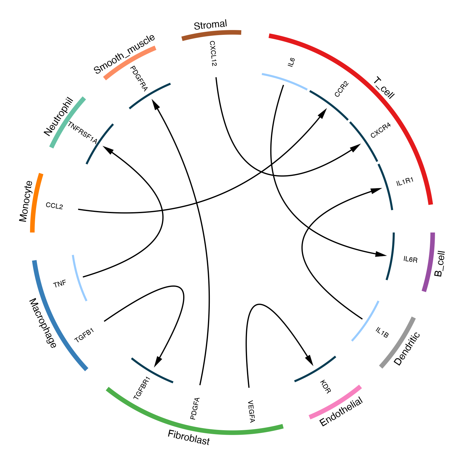
Basic circos plot showing ligand-receptor interactions between cell types
Understanding the Circos Plot
The circos plot encodes multiple dimensions:
- Outer ring: Cell types (colored sectors)
- Inner ring: Gene names (ligands and receptors)
- Arrows: Communication direction (ligand → receptor)
- Arrow width: Expression level of ligand
- Arrow head width: Expression level of receptor
Customized Circos Plot
# Custom arrow properties based on expression
LRPlot(
  data = lr_data,
  datatype = "mean count",
  cell_col = cell_colors,
  transparency = 0.3,
  link.arr.type = "big.arrow",
  track.height_1 = circlize::uh(3, "mm"),
  track.height_2 = circlize::uh(15, "mm"),
  text.vjust = "0.5cm"
)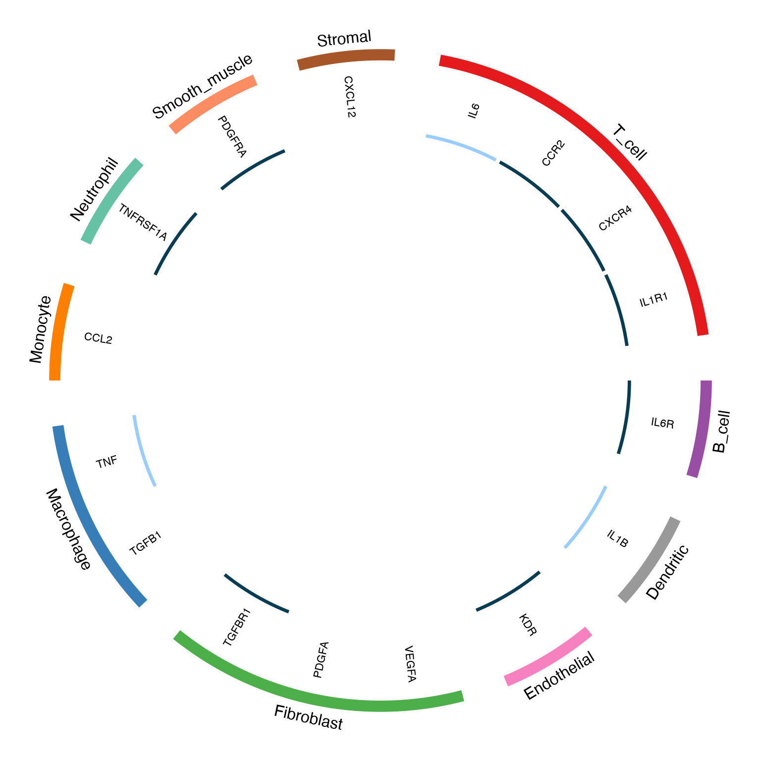
Customized circos plot with adjusted arrow properties
NetView: Network Visualization
Basic Network Plot
The NetView() function creates a network graph showing
overall communication patterns between cell types.
g <- NetView(
  data = lr_data,
  col = cell_colors,
  vertex.size = 30,
  vertex.label.cex = 0.8,
  edge.max.width = 8,
  edge.curved = 0.2,
  arrow.width = 1.5,
  margin = 0.2
)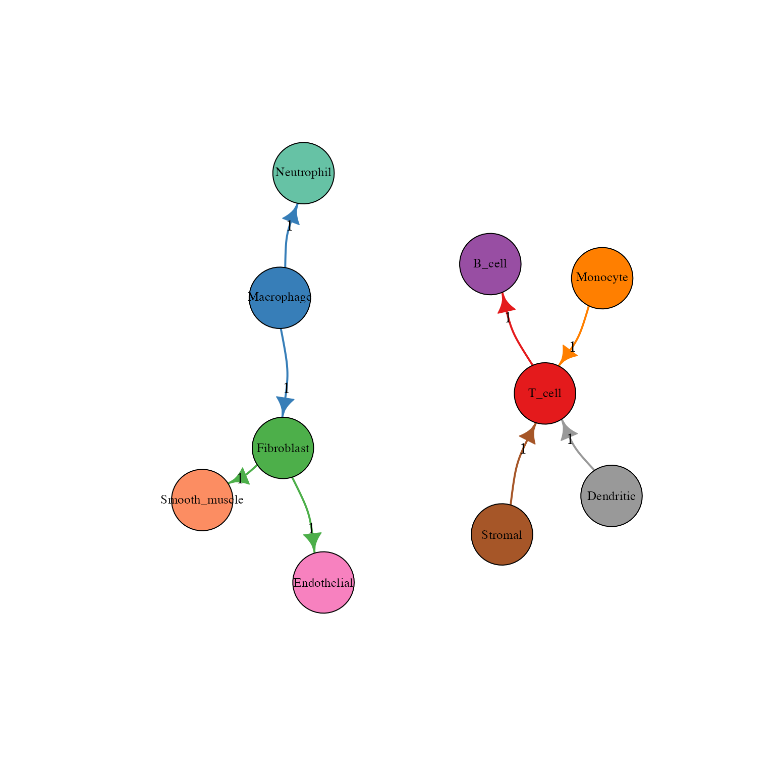
Network view of cell-cell communication
Understanding the Network
- Nodes: Cell types (size can represent number of interactions)
- Edges: Communication channels between cells
- Edge width: Number of L-R pairs
- Edge color: Source cell type color
- Arrows: Direction of communication
Customized Network with Labels
g <- NetView(
  data = lr_data,
  col = cell_colors,
  vertex.size = 35,
  vertex.label.cex = 0.9,
  vertex.label.color = "white",
  edge.max.width = 10,
  edge.curved = 0.3,
  arrow.width = 2,
  edge.label.cex = 0.7,
  edge.label.color = "darkgray",
  label = TRUE,
  margin = 0.15
)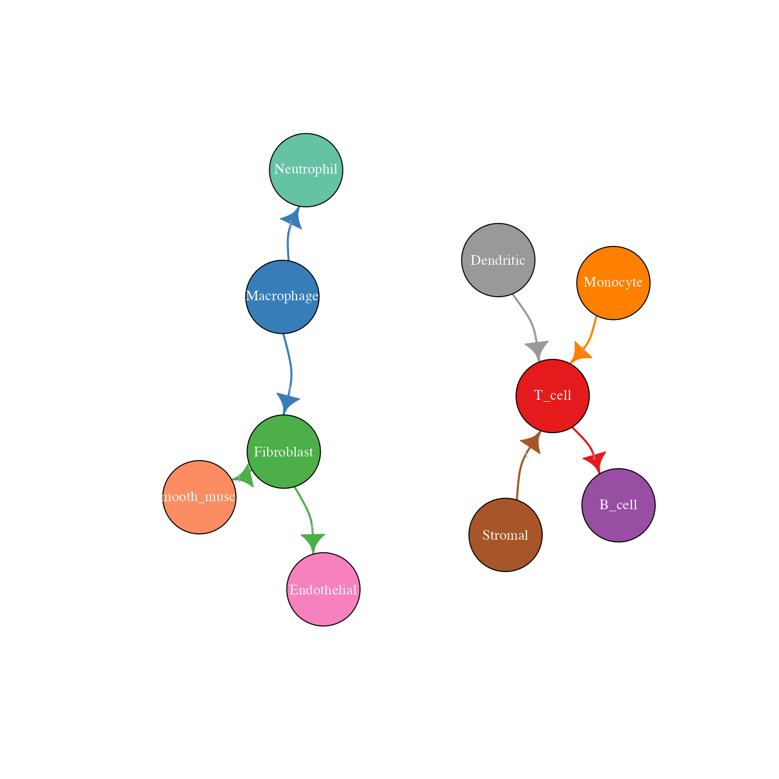
Network plot with edge labels showing interaction counts
DEG Data Visualization
For differential expression results, the visualization changes to show up/down regulation:
# Create DEG-style data
lr_deg <- data.frame(
  ligand = c("TGFB1", "IL6", "CCL2", "TNF"),
  receptor = c("TGFBR1", "IL6R", "CCR2", "TNFRSF1A"),
  cell_from = c("Macrophage", "T_cell", "Monocyte", "Macrophage"),
  cell_to = c("Fibroblast", "B_cell", "T_cell", "Neutrophil"),
  cell_from_logFC = c(2.5, -1.8, 1.2, 3.0),
  cell_to_logFC = c(1.8, 2.1, -0.8, 1.5),
  comm_type = c("growth_factor", "cytokine", "chemokine", "cytokine"),
  stringsAsFactors = FALSE
)
LRPlot(
  data = lr_deg,
  datatype = "DEG",
  cell_col = cell_colors,
  transparency = 0.4
)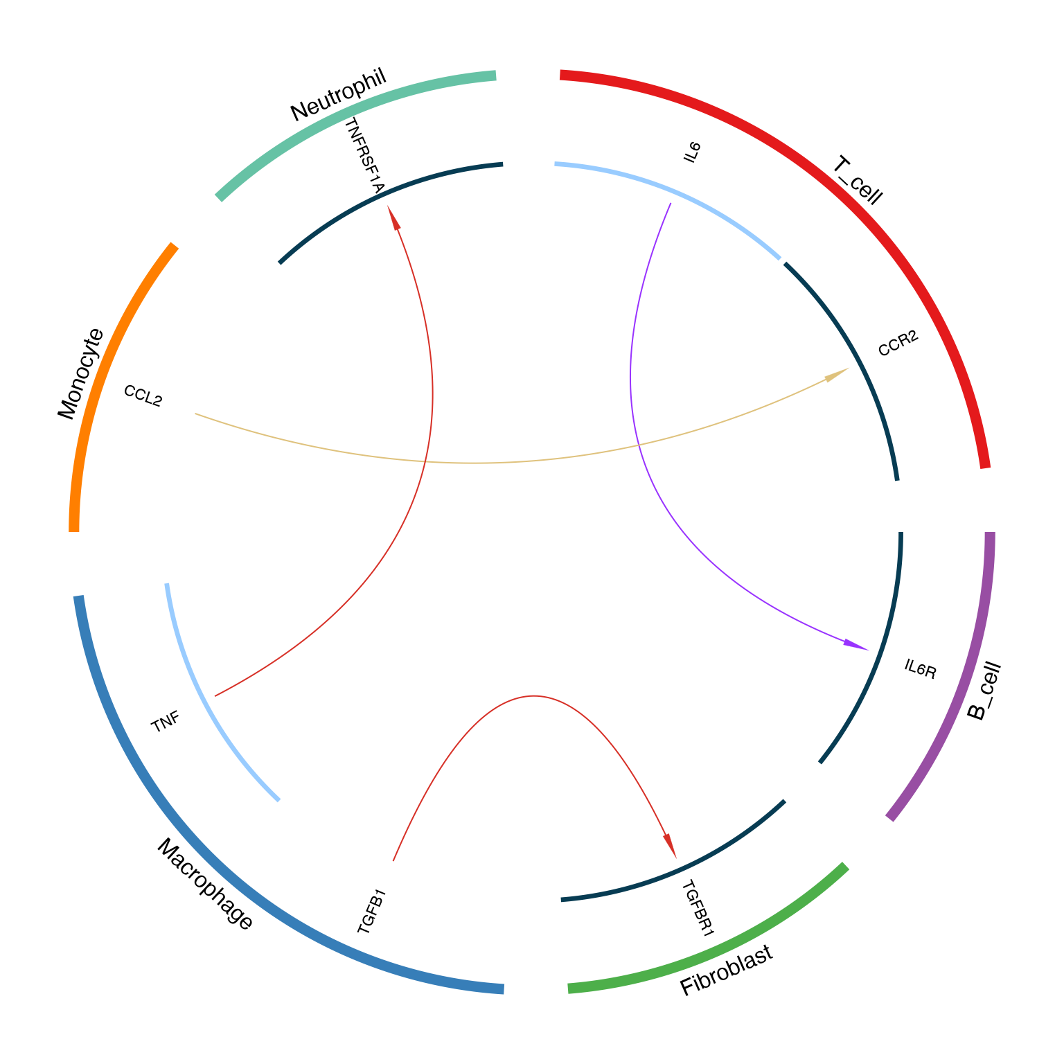
Circos plot for DEG data showing up/down regulation
Arrow color coding for DEG:
| Ligand | Receptor | Arrow Color |
|---|---|---|
| ↑ Up | ↑ Up | Red (#d73027) |
| ↑ Up | ↓ Down | Yellow (#dfc27d) |
| ↓ Down | ↑ Up | Purple (#9933ff) |
| ↓ Down | ↓ Down | Cyan (#00ccff) |
Color Recommendations
Scientific Color Palettes
# Display recommended palettes
par(mfrow = c(1, 3), mar = c(1, 1, 2, 1))

# Option 1: Set1 from RColorBrewer
pal1 <- c("#E41A1C", "#377EB8", "#4DAF4A", "#984EA3", "#FF7F00", "#A65628")
barplot(rep(1, 6), col = pal1, border = NA, main = "Set1 Palette", axes = FALSE)

# Option 2: Paired
pal2 <- c("#A6CEE3", "#1F78B4", "#B2DF8A", "#33A02C", "#FB9A99", "#E31A1C")
barplot(rep(1, 6), col = pal2, border = NA, main = "Paired Palette", axes = FALSE)

# Option 3: Dark2
pal3 <- c("#1B9E77", "#D95F02", "#7570B3", "#E7298A", "#66A61E", "#E6AB02")
barplot(rep(1, 6), col = pal3, border = NA, main = "Dark2 Palette", axes = FALSE)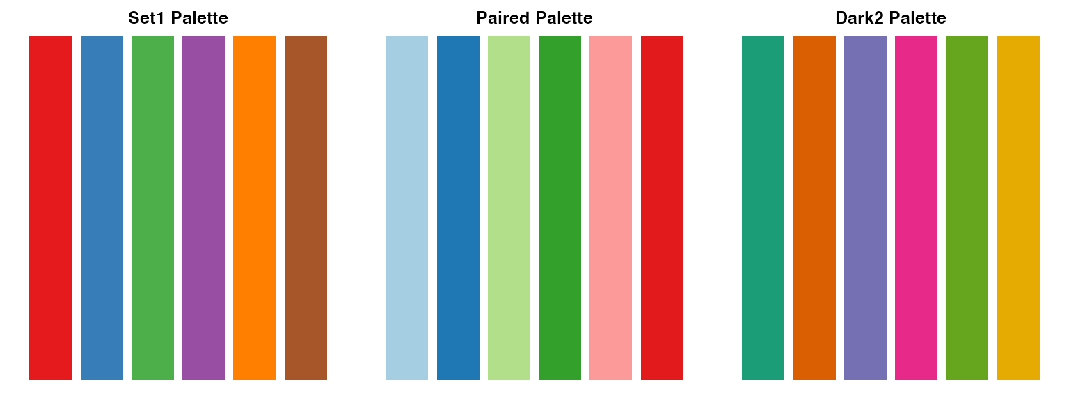
Publication-Ready Export
# PDF export for vector graphics
pdf("communication_circos.pdf", width = 10, height = 10)
LRPlot(lr_data, datatype = "mean count", cell_col = cell_colors)
dev.off()

# PNG export for high-resolution raster
png("communication_network.png", width = 3000, height = 3000, res = 300)
NetView(lr_data, col = cell_colors, vertex.size = 30)
dev.off()
Tips and Best Practices
- Limit pairs for clarity: Show top 20-30 pairs in LRPlot for readability
- Consistent colors: Use the same cell colors across all plots
- Meaningful order: Sort data by expression/significance before plotting
- Vector formats: Use PDF for publication-quality figures
- Color blindness: Consider colorblind-friendly palettes
Session Info
sessionInfo()
#> R version 4.4.0 (2024-04-24)
#> Platform: aarch64-apple-darwin20
#> Running under: macOS 15.6.1
#>
#> Matrix products: default
#> BLAS:   /Library/Frameworks/R.framework/Versions/4.4-arm64/Resources/lib/libRblas.0.dylib
#> LAPACK: /Library/Frameworks/R.framework/Versions/4.4-arm64/Resources/lib/libRlapack.dylib;  LAPACK version 3.12.0
#>
#> locale:
#> [1] C
#>
#> time zone: Asia/Shanghai
#> tzcode source: internal
#>
#> attached base packages:
#> [1] stats     graphics  grDevices utils     datasets  methods   base
#>
#> other attached packages:
#> [1] dplyr_1.1.4 iTALK_0.1.1
#>
#> loaded via a namespace (and not attached):
#>   [1] RColorBrewer_1.1-3          RcppArmadillo_15.2.3-1
#>   [3] jsonlite_2.0.0              shape_1.4.6.1
#>   [5] magrittr_2.0.4              modeltools_0.2-24
#>   [7] farver_2.1.2                rmarkdown_2.30
#>   [9] GlobalOptions_0.1.3         fs_1.6.6
#>  [11] zlibbioc_1.52.0             ragg_1.5.0
#>  [13] vctrs_0.7.0                 Cairo_1.7-0
#>  [15] fastICA_1.2-7               scde_2.34.0
#>  [17] progress_1.2.3              htmltools_0.5.9
#>  [19] S4Arrays_1.6.0              curl_7.0.0
#>  [21] SparseArray_1.6.2           sass_0.4.10
#>  [23] bslib_0.9.0                 HSMMSingleCell_1.26.0
#>  [25] htmlwidgets_1.6.4           desc_1.4.3
#>  [27] plyr_1.8.9                  sandwich_3.1-1
#>  [29] zoo_1.8-15                  cachem_1.1.0
#>  [31] igraph_2.2.1                lifecycle_1.0.5
#>  [33] pkgconfig_2.0.3             Matrix_1.7-4
#>  [35] R6_2.6.1                    fastmap_1.2.0
#>  [37] GenomeInfoDbData_1.2.13     MatrixGenerics_1.18.1
#>  [39] digest_0.6.39               numDeriv_2016.8-1.1
#>  [41] pcaMethods_1.98.0           colorspace_2.1-2
#>  [43] miscTools_0.6-28            S4Vectors_0.44.0
#>  [45] DESeq2_1.46.0               irlba_2.3.5.1
#>  [47] textshaping_1.0.4           GenomicRanges_1.58.0
#>  [49] extRemes_2.2-1              RMTstat_0.3.1
#>  [51] mgcv_1.9-3                  httr_1.4.7
#>  [53] abind_1.4-8                 compiler_4.4.0
#>  [55] brew_1.0-10                 S7_0.2.1
#>  [57] BiocParallel_1.40.2         viridis_0.6.5
#>  [59] MASS_7.3-65                 quantreg_6.1
#>  [61] MAST_1.32.0                 DelayedArray_0.32.0
#>  [63] rjson_0.2.23                tools_4.4.0
#>  [65] otel_0.2.0                  DDRTree_0.1.5
#>  [67] nnet_7.3-20                 glue_1.8.0
#>  [69] nlme_3.1-168                grid_4.4.0
#>  [71] Rtsne_0.17                  cluster_2.1.8.1
#>  [73] reshape2_1.4.5              generics_0.1.4
#>  [75] gtable_0.3.6                monocle_2.34.0
#>  [77] tidyr_1.3.2                 hms_1.1.4
#>  [79] data.table_1.18.0           flexmix_2.3-20
#>  [81] XVector_0.46.0              BiocGenerics_0.52.0
#>  [83] RANN_2.6.2                  pillar_1.11.1
#>  [85] stringr_1.6.0               Lmoments_1.3-2
#>  [87] limma_3.62.2                circlize_0.4.17
#>  [89] splines_4.4.0               Rook_1.2
#>  [91] lattice_0.22-7              survival_3.8-3
#>  [93] SparseM_1.84-2              gamlss.data_6.0-7
#>  [95] tidyselect_1.2.1            SingleCellExperiment_1.28.1
#>  [97] locfit_1.5-9.12             pbapply_1.7-4
#>  [99] randomcoloR_1.1.0.1         knitr_1.51
#> [101] gridExtra_2.3               V8_8.0.1
#> [103] IRanges_2.40.1              edgeR_4.4.2
#> [105] SummarizedExperiment_1.36.0 stats4_4.4.0
#> [107] xfun_0.56                   Biobase_2.66.0
#> [109] statmod_1.5.1               matrixStats_1.5.0
#> [111] pheatmap_1.0.13             leidenbase_0.1.36
#> [113] stringi_1.8.7               VGAM_1.1-14
#> [115] UCSC.utils_1.2.0            statnet.common_4.13.0
#> [117] yaml_2.3.12                 evaluate_1.0.5
#> [119] codetools_0.2-20            bbmle_1.0.25.1
#> [121] DEsingle_1.26.0             tibble_3.3.1
#> [123] cli_3.6.5                   systemfonts_1.3.1
#> [125] jquerylib_0.1.4             network_1.19.0
#> [127] dichromat_2.0-0.1           pscl_1.5.9
#> [129] Rcpp_1.1.1                  GenomeInfoDb_1.42.3
#> [131] coda_0.19-4.1               bdsmatrix_1.3-7
#> [133] parallel_4.4.0              MatrixModels_0.5-4
#> [135] pkgdown_2.1.3               ggplot2_4.0.1
#> [137] prettyunits_1.2.0           gamlss.dist_6.1-1
#> [139] viridisLite_0.4.2           mvtnorm_1.3-3
#> [141] slam_0.1-55                 scales_1.4.0
#> [143] gamlss_5.5-0                purrr_1.2.1
#> [145] crayon_1.5.3                combinat_0.0-8
#> [147] distillery_1.2-2            maxLik_1.5-2.1
#> [149] rlang_1.1.7