Algorithm and Statistical Methods

Overview

This vignette describes the statistical methods and algorithms implemented in iTALK for intercellular communication analysis.

Ligand-Receptor Database

Database Structure

iTALK includes a curated database of 2,649 ligand-receptor pairs categorized into four functional groups:

library(iTALK)

# Access the internal database
db <- iTALK:::database

cat("Total L-R pairs:", nrow(db), "\n\n")
#> Total L-R pairs: 2649
cat("Categories:\n")
#> Categories:
print(table(db$Classification))
#> 
#>    checkpoint      cytokine growth factor         other 
#>            32           327           227          2063

Database Sources

The database integrates information from:

Cytokines - Zhang et al., 2007; Cameron et al., 2000-2013
Checkpoint molecules - Auslander et al., 2018
Ligand-receptor pairs - Ramilowski et al., Nature Communications, 2015

# Database columns
cat("Database columns:", paste(colnames(db), collapse = ", "), "\n\n")
#> Database columns: Pair.Name, Ligand.ApprovedSymbol, Ligand.Name, Receptor.ApprovedSymbol, Receptor.Name, Classification

# Example entries
head(db[, c("Ligand.ApprovedSymbol", "Receptor.ApprovedSymbol", "Classification")])
#>   Ligand.ApprovedSymbol Receptor.ApprovedSymbol Classification
#> 1                   A2M                    LRP1          other
#> 2                 AANAT                  MTNR1A          other
#> 3                 AANAT                  MTNR1B          other
#> 4                   ACE                   AGTR2          other
#> 5                   ACE                  BDKRB2          other
#> 6                ADAM10                     AXL          other

Statistical Methods for Differential Expression

Method Comparison

iTALK supports seven statistical methods for identifying differentially expressed genes:

Method	Model	Best For	Reference
Wilcox	Wilcoxon rank-sum	General purpose	-
DESeq2	Negative binomial	Bulk RNA-seq	Love et al., 2014
edgeR	Negative binomial + EB	Bulk RNA-seq	McCarthy et al., 2012
MAST	Two-part hurdle	scRNA-seq	Finak et al., 2015
monocle	Census-based	Trajectory analysis	Qiu et al., 2017
SCDE	Bayesian	scRNA-seq	Kharchenko et al., 2014
DEsingle	Zero-inflated NB	Dropout modeling	Miao et al., 2018

Wilcoxon Rank-Sum Test

The default method uses the Wilcoxon rank-sum test (Mann-Whitney U test):

$W = \sum_{i=1}^{n_1} R_i - \frac{n_1(n_1+1)}{2}$

Where $R_i$ is the rank of observation $i$ in the combined sample.

Log Fold Change Calculation:

For raw counts: $\log_2 FC = \log_2 \frac{\bar{x}_1 + \epsilon}{\bar{x}_2 + \epsilon}$

Where $\epsilon = 10^{-9}$ prevents division by zero.

For log-transformed data: $\log_2 FC = \bar{x}_1 - \bar{x}_2$

# Example: Wilcoxon test
deg_result <- DEG(
  data = expression_data,
  method = "Wilcox",
  q_cut = 0.05,
  contrast = c("Treatment", "Control")
)

DESeq2 Model

DESeq2 uses a negative binomial generalized linear model:

$K_{ij} \sim NB(\mu_{ij}, \alpha_i)$

$\mu_{ij} = s_j q_{ij}$

$\log_2 q_{ij} = \sum_r x_{jr} \beta_{ir}$

Where: - $K_{ij}$ = read count for gene $i$ in sample $j$ - $s_j$ = size factor for sample $j$ - $\alpha_i$ = dispersion for gene $i$ - $\beta_{ir}$ = log2 fold change

MAST Hurdle Model

MAST uses a two-part hurdle model for scRNA-seq data:

Part 1 (Discrete): Logistic regression for detection $\log \frac{P(Z_g = 1)}{P(Z_g = 0)} = X\beta_D$

Part 2 (Continuous): Linear model for expression given detection $E[Y_g | Z_g = 1] = X\beta_C$

The combined test statistic follows a $\chi^2$ distribution with 2 degrees of freedom.

L-R Pair Detection Algorithm

Workflow

┌─────────────────┐
│  Gene List(s)   │
│  (expr/DEG)     │
└────────┬────────┘
         │
         ▼
┌─────────────────┐
│ Species Check   │──► Auto-conversion if needed
└────────┬────────┘
         │
         ▼
┌─────────────────┐
│ Database Match  │
│ Ligand ∩ Recep  │
└────────┬────────┘
         │
         ▼
┌─────────────────┐
│ Annotate Pairs  │
│ + Cell Types    │
└────────┬────────┘
         │
         ▼
┌─────────────────┐
│ Filter & Output │
└─────────────────┘

Matching Algorithm

For “mean count” datatype:

# Pseudocode
ligand_genes <- intersect(input_genes, database$Ligand)
receptor_genes <- intersect(input_genes, database$Receptor)
pairs <- database[database$Ligand %in% ligand_genes & 
                  database$Receptor %in% receptor_genes, ]

For “DEG” datatype, additional filtering removes pairs where both ligand and receptor are not differentially expressed (logFC = 0.0001 placeholder).

Multiple Testing Correction

All p-values are adjusted using the Benjamini-Hochberg procedure:

$q_i = \min\left(1, \frac{p_i \cdot m}{i}\right)$

Where: - $p_i$ = i-th smallest p-value - $m$ = total number of tests - $q_i$ = adjusted p-value (FDR)

# Demonstration of BH correction
set.seed(42)
p_values <- c(runif(50, 0, 0.01), runif(50, 0.01, 1))  # Mix of significant and non-significant

q_values <- p.adjust(p_values, method = "BH")

# Visualize
par(mfrow = c(1, 2))
hist(p_values, breaks = 20, main = "Raw P-values", xlab = "P-value", col = "steelblue")
hist(q_values, breaks = 20, main = "BH-adjusted Q-values", xlab = "Q-value", col = "coral")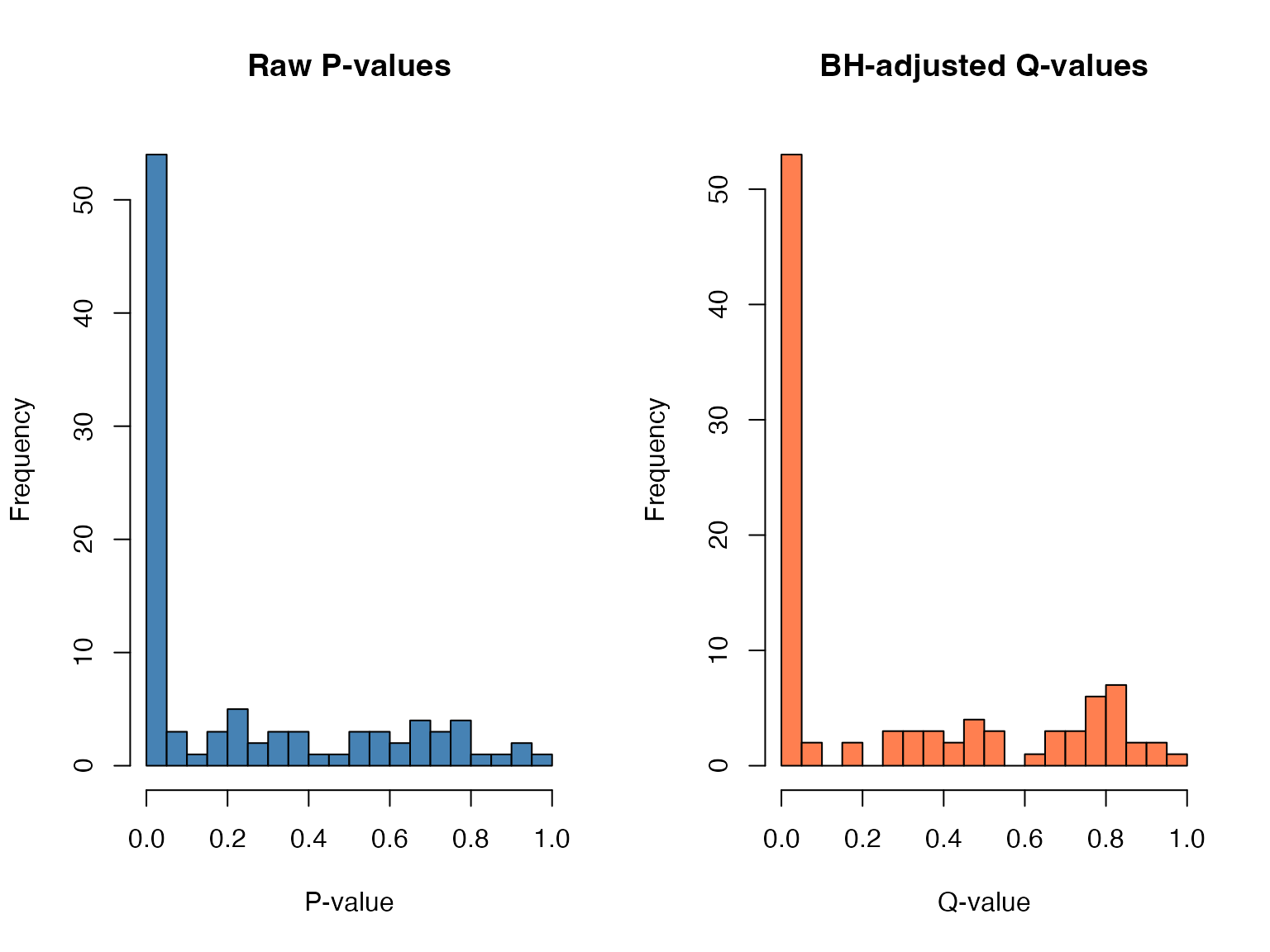

Communication Strength Metrics

Expression-based Scoring

For mean count analysis, communication strength is proportional to:

$S_{LR} = \bar{E}_L \times \bar{E}_R$

Where $\bar{E}_L$ and $\bar{E}_R$ are mean expression levels of ligand and receptor.

Fold Change-based Scoring

For DEG analysis:

$S_{LR} = |FC_L| \times |FC_R| \times \text{sign}(FC_L \times FC_R)$

This captures both magnitude and directionality of changes.

Network Construction

Cell-cell communication networks are constructed using:

Nodes = Cell types
Edges = Number of L-R pairs between cell types
Edge weights = Communication frequency or strength

library(igraph)

# Example network construction
edges <- data.frame(
  from = c("T_cell", "T_cell", "Macrophage", "Dendritic"),
  to = c("Macrophage", "B_cell", "T_cell", "T_cell"),
  weight = c(15, 8, 12, 6)
)

g <- graph_from_data_frame(edges, directed = TRUE)
E(g)$width <- E(g)$weight / 3

plot(g, 
     vertex.size = 30,
     vertex.color = "lightblue",
     edge.arrow.size = 0.5,
     main = "Cell Communication Network")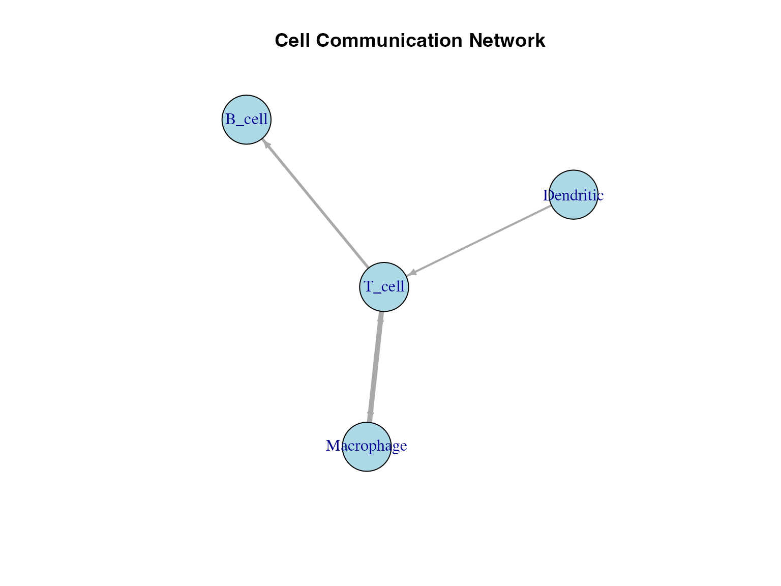

Computational Complexity

Operation	Time Complexity	Space Complexity
rawParse	O(n × g)	O(c × g)
FindLR	O(g × d)	O(p)
DEG (Wilcox)	O(n × g)	O(g)
LRPlot	O(p)	O(p)
NetView	O(c²)	O(c²)

Where: - n = number of cells - g = number of genes - c = number of cell types - d = database size - p = number of pairs

References

Love MI, Huber W, Anders S. Moderated estimation of fold change and dispersion for RNA-seq data with DESeq2. Genome Biology. 2014;15:550.
Finak G, et al. MAST: a flexible statistical framework for assessing transcriptional changes and characterizing heterogeneity in single-cell RNA sequencing data. Genome Biology. 2015;16:278.
Wang Y, et al. iTALK: an R Package to Characterize and Illustrate Intercellular Communication. bioRxiv. 2019;507871.

Session Info

sessionInfo()
#> R version 4.4.0 (2024-04-24)
#> Platform: aarch64-apple-darwin20
#> Running under: macOS 15.6.1
#> 
#> Matrix products: default
#> BLAS:   /Library/Frameworks/R.framework/Versions/4.4-arm64/Resources/lib/libRblas.0.dylib 
#> LAPACK: /Library/Frameworks/R.framework/Versions/4.4-arm64/Resources/lib/libRlapack.dylib;  LAPACK version 3.12.0
#> 
#> locale:
#> [1] C
#> 
#> time zone: Asia/Shanghai
#> tzcode source: internal
#> 
#> attached base packages:
#> [1] stats     graphics  grDevices utils     datasets  methods   base     
#> 
#> other attached packages:
#> [1] igraph_2.2.1 iTALK_0.1.1 
#> 
#> loaded via a namespace (and not attached):
#>   [1] RColorBrewer_1.1-3          RcppArmadillo_15.2.3-1     
#>   [3] jsonlite_2.0.0              shape_1.4.6.1              
#>   [5] magrittr_2.0.4              modeltools_0.2-24          
#>   [7] farver_2.1.2                rmarkdown_2.30             
#>   [9] GlobalOptions_0.1.3         fs_1.6.6                   
#>  [11] zlibbioc_1.52.0             ragg_1.5.0                 
#>  [13] vctrs_0.7.0                 Cairo_1.7-0                
#>  [15] fastICA_1.2-7               scde_2.34.0                
#>  [17] progress_1.2.3              htmltools_0.5.9            
#>  [19] S4Arrays_1.6.0              curl_7.0.0                 
#>  [21] SparseArray_1.6.2           sass_0.4.10                
#>  [23] bslib_0.9.0                 HSMMSingleCell_1.26.0      
#>  [25] htmlwidgets_1.6.4           desc_1.4.3                 
#>  [27] plyr_1.8.9                  sandwich_3.1-1             
#>  [29] zoo_1.8-15                  cachem_1.1.0               
#>  [31] lifecycle_1.0.5             pkgconfig_2.0.3            
#>  [33] Matrix_1.7-4                R6_2.6.1                   
#>  [35] fastmap_1.2.0               GenomeInfoDbData_1.2.13    
#>  [37] MatrixGenerics_1.18.1       digest_0.6.39              
#>  [39] numDeriv_2016.8-1.1         pcaMethods_1.98.0          
#>  [41] colorspace_2.1-2            miscTools_0.6-28           
#>  [43] S4Vectors_0.44.0            DESeq2_1.46.0              
#>  [45] irlba_2.3.5.1               textshaping_1.0.4          
#>  [47] GenomicRanges_1.58.0        extRemes_2.2-1             
#>  [49] RMTstat_0.3.1               mgcv_1.9-3                 
#>  [51] httr_1.4.7                  abind_1.4-8                
#>  [53] compiler_4.4.0              brew_1.0-10                
#>  [55] S7_0.2.1                    BiocParallel_1.40.2        
#>  [57] viridis_0.6.5               MASS_7.3-65                
#>  [59] quantreg_6.1                MAST_1.32.0                
#>  [61] DelayedArray_0.32.0         rjson_0.2.23               
#>  [63] tools_4.4.0                 otel_0.2.0                 
#>  [65] DDRTree_0.1.5               nnet_7.3-20                
#>  [67] glue_1.8.0                  nlme_3.1-168               
#>  [69] grid_4.4.0                  Rtsne_0.17                 
#>  [71] cluster_2.1.8.1             reshape2_1.4.5             
#>  [73] generics_0.1.4              gtable_0.3.6               
#>  [75] monocle_2.34.0              tidyr_1.3.2                
#>  [77] hms_1.1.4                   data.table_1.18.0          
#>  [79] flexmix_2.3-20              XVector_0.46.0             
#>  [81] BiocGenerics_0.52.0         RANN_2.6.2                 
#>  [83] pillar_1.11.1               stringr_1.6.0              
#>  [85] Lmoments_1.3-2              limma_3.62.2               
#>  [87] circlize_0.4.17             splines_4.4.0              
#>  [89] dplyr_1.1.4                 Rook_1.2                   
#>  [91] lattice_0.22-7              survival_3.8-3             
#>  [93] SparseM_1.84-2              gamlss.data_6.0-7          
#>  [95] tidyselect_1.2.1            SingleCellExperiment_1.28.1
#>  [97] locfit_1.5-9.12             pbapply_1.7-4              
#>  [99] randomcoloR_1.1.0.1         knitr_1.51                 
#> [101] gridExtra_2.3               V8_8.0.1                   
#> [103] IRanges_2.40.1              edgeR_4.4.2                
#> [105] SummarizedExperiment_1.36.0 stats4_4.4.0               
#> [107] xfun_0.56                   Biobase_2.66.0             
#> [109] statmod_1.5.1               matrixStats_1.5.0          
#> [111] pheatmap_1.0.13             leidenbase_0.1.36          
#> [113] stringi_1.8.7               VGAM_1.1-14                
#> [115] UCSC.utils_1.2.0            statnet.common_4.13.0      
#> [117] yaml_2.3.12                 evaluate_1.0.5             
#> [119] codetools_0.2-20            bbmle_1.0.25.1             
#> [121] DEsingle_1.26.0             tibble_3.3.1               
#> [123] cli_3.6.5                   systemfonts_1.3.1          
#> [125] jquerylib_0.1.4             network_1.19.0             
#> [127] dichromat_2.0-0.1           pscl_1.5.9                 
#> [129] Rcpp_1.1.1                  GenomeInfoDb_1.42.3        
#> [131] coda_0.19-4.1               bdsmatrix_1.3-7            
#> [133] parallel_4.4.0              MatrixModels_0.5-4         
#> [135] pkgdown_2.1.3               ggplot2_4.0.1              
#> [137] prettyunits_1.2.0           gamlss.dist_6.1-1          
#> [139] viridisLite_0.4.2           mvtnorm_1.3-3              
#> [141] slam_0.1-55                 scales_1.4.0               
#> [143] gamlss_5.5-0                purrr_1.2.1                
#> [145] crayon_1.5.3                combinat_0.0-8             
#> [147] distillery_1.2-2            maxLik_1.5-2.1             
#> [149] rlang_1.1.7

Zaoqu Liu

2026-01-23