Introduction
iTALK (intercellular communication analysis toolkit) is an R package designed to characterize and visualize cell-cell communication from transcriptomic data. This vignette provides a quick introduction to the core functionality.
Installation
# From R-Universe (recommended)
install.packages("iTALK", repos = "https://zaoqu-liu.r-universe.dev")

# From GitHub
remotes::install_github("Zaoqu-Liu/iTALK")
Load Package and Create Example Data
library(iTALK)
library(dplyr)

# Access database to get real ligand-receptor pairs
db <- iTALK:::database
cyto_db <- db[db$Classification == "cytokine", ]

# Get some real ligands and receptors from the database
ligands <- head(unique(cyto_db$Ligand.ApprovedSymbol), 10)
receptors <- head(unique(cyto_db$Receptor.ApprovedSymbol), 10)
genes <- unique(c(ligands, receptors))

cat("Using genes from database:\n")
#> Using genes from database:
cat("Ligands:", paste(ligands, collapse = ", "), "\n")
#> Ligands: CCL11, CCL13, CCL14, CCL15, CCL16, CCL17, CCL18, CCL19, CCL1, CCL20
cat("Receptors:", paste(receptors, collapse = ", "), "\n\n")
#> Receptors: ACKR2, ACKR4, CCR2, CCR3, CCR5, CXCR3, CCR1, CCR9, CCR8, HRH4

# Create synthetic expression data
set.seed(42)
n_cells <- 200
cell_types <- c("T_cell", "B_cell", "Macrophage", "Dendritic", "NK_cell")

data <- data.frame(
  cell_type = sample(cell_types, n_cells, replace = TRUE)
)

# Add gene expression
for (gene in genes) {
  data[[gene]] <- rpois(n_cells, lambda = sample(5:25, 1))
}

cat("Data dimensions:", nrow(data), "cells x", ncol(data), "columns\n")
#> Data dimensions: 200 cells x 21 columns
cat("Cell types:", paste(unique(data$cell_type), collapse = ", "), "\n")
#> Cell types: T_cell, NK_cell, B_cell, Dendritic, Macrophage
head(data[, 1:6])
#>   cell_type CCL11 CCL13 CCL14 CCL15 CCL16
#> 1    T_cell    11    22    21     7    13
#> 2   NK_cell    20    14    22     7     8
#> 3    T_cell     8    22    20     4     8
#> 4    T_cell    11    28    27    12    14
#> 5    B_cell    17    30    34     6    12
#> 6 Dendritic    12    19    18     7     7
Workflow 1: Highly Expressed Gene Analysis
Step 1: Parse Expression Data
Identify the top expressed genes in each cell type:
# Get top 50% highly expressed genes per cell type
highly_expr <- rawParse(data, top_genes = 50, stats = "mean")

cat("\nTop expressed genes found:", nrow(highly_expr), "\n")
#>
#> Top expressed genes found: 50
cat("Cell types:", paste(unique(highly_expr$cell_type), collapse = ", "), "\n\n")
#> Cell types: T_cell, NK_cell, B_cell, Dendritic, Macrophage
head(highly_expr)
#>    gene    exprs cell_type
#> 1 CCL14 25.65306    T_cell
#> 2 CXCR3 24.55102    T_cell
#> 3 CCL13 24.24490    T_cell
#> 4  CCR8 23.89796    T_cell
#> 5  HRH4 19.02041    T_cell
#> 6 ACKR4 17.63265    T_cell
Step 2: Find Ligand-Receptor Pairs
# Find ligand-receptor pairs from cytokine category
lr_pairs <- FindLR(
  data_1 = highly_expr,
  datatype = "mean count",
  comm_type = "cytokine"
)

cat("Found", nrow(lr_pairs), "ligand-receptor pairs\n\n")
#> Found 243 ligand-receptor pairs
if (nrow(lr_pairs) > 0) {
  head(lr_pairs)
}
#>   ligand receptor cell_from_mean_exprs cell_from cell_to_mean_exprs    cell_to
#> 1  CCL11    ACKR2             13.26531    T_cell           14.34694     T_cell
#> 2  CCL11    ACKR2             13.26531    T_cell           14.58974    NK_cell
#> 3  CCL11    ACKR2             13.26531    T_cell           15.08889     B_cell
#> 4  CCL11    ACKR2             13.26531    T_cell           13.60000  Dendritic
#> 5  CCL11    ACKR2             13.26531    T_cell           13.25926 Macrophage
#> 6  CCL11    ACKR2             12.30769   NK_cell           14.34694     T_cell
#>   comm_type
#> 1  cytokine
#> 2  cytokine
#> 3  cytokine
#> 4  cytokine
#> 5  cytokine
#> 6  cytokine
Step 3: Visualize with Circos Plot
# Define cell type colors
cell_col <- c(
  "T_cell" = "#E41A1C",
  "B_cell" = "#377EB8",
  "Macrophage" = "#4DAF4A",
  "Dendritic" = "#984EA3",
  "NK_cell" = "#FF7F00"
)

# Create circos plot
if (nrow(lr_pairs) > 0) {
  # Take top pairs for cleaner visualization
  plot_data <- lr_pairs[1:min(20, nrow(lr_pairs)), ]

  LRPlot(
    data = plot_data,
    datatype = "mean count",
    cell_col = cell_col,
    transparency = 0.5,
    link.arr.type = "triangle"
  )
}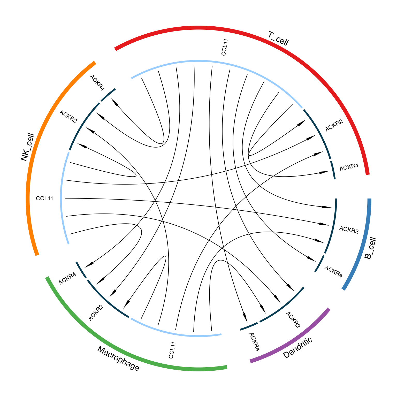
Circos plot showing ligand-receptor interactions between cell types
Workflow 2: Multi-Category Analysis
You can analyze different communication types separately:
# Communication categories in database
comm_types <- c("cytokine", "growth factor", "checkpoint", "other")

# Analyze each category
results_list <- list()
for (comm in comm_types) {
  lr <- FindLR(highly_expr, datatype = "mean count", comm_type = comm)
  if (nrow(lr) > 0) {
    results_list[[comm]] <- lr
    cat(comm, ":", nrow(lr), "pairs\n")
  }
}
#> cytokine : 243 pairs
Workflow 3: Using the Ligand-Receptor Database
iTALK includes a curated database of ligand-receptor pairs:
# Access the built-in database
data(database)

cat("Database contains", nrow(database), "ligand-receptor pairs\n\n")
#> Database contains 2649 ligand-receptor pairs
cat("Categories:", paste(unique(database$Classification), collapse = ", "), "\n\n")
#> Categories: other, checkpoint, cytokine, growth factor

# Preview
head(database[, c("Pair.Name", "Ligand.ApprovedSymbol", "Receptor.ApprovedSymbol", "Classification")])
#>      Pair.Name Ligand.ApprovedSymbol Receptor.ApprovedSymbol Classification
#> 1     A2M_LRP1                   A2M                    LRP1          other
#> 2 AANAT_MTNR1A                 AANAT                  MTNR1A          other
#> 3 AANAT_MTNR1B                 AANAT                  MTNR1B          other
#> 4    ACE_AGTR2                   ACE                   AGTR2          other
#> 5   ACE_BDKRB2                   ACE                  BDKRB2          other
#> 6   ADAM10_AXL                ADAM10                     AXL          other
Summary
This quick start covered:
- Data preparation - Expression matrix with cell type annotations
- Gene parsing - Identifying highly expressed genes per cell type
- L-R detection - Finding ligand-receptor pairs from the database
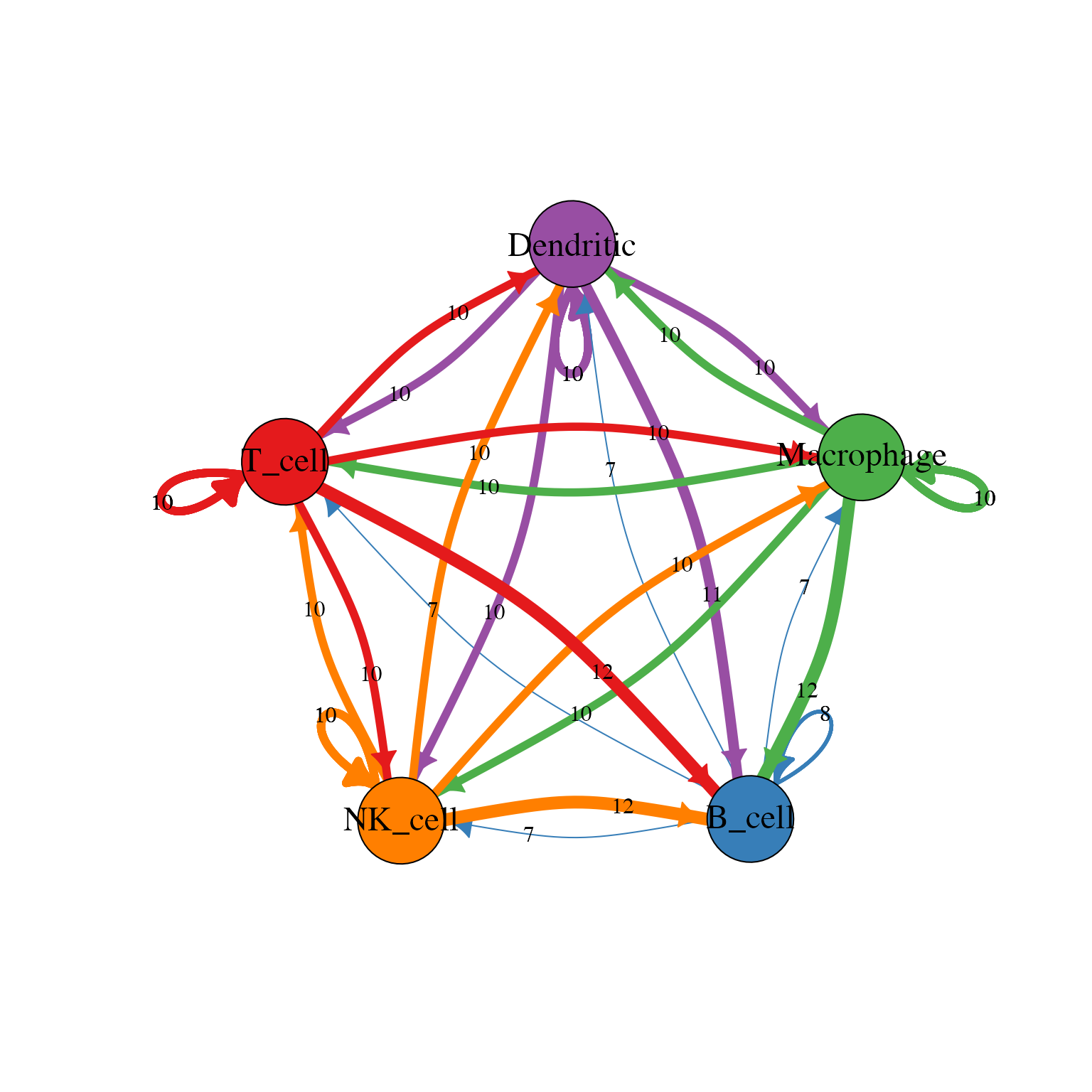
- Visualization - Circos and network plots
For more advanced usage, see:
-
vignette("algorithm")- Statistical methods and database -
vignette("species-conversion")- Cross-species analysis -
vignette("visualization")- Comprehensive visualization guide
Session Info
sessionInfo()
#> R version 4.4.0 (2024-04-24)
#> Platform: aarch64-apple-darwin20
#> Running under: macOS 15.6.1
#>
#> Matrix products: default
#> BLAS:   /Library/Frameworks/R.framework/Versions/4.4-arm64/Resources/lib/libRblas.0.dylib
#> LAPACK: /Library/Frameworks/R.framework/Versions/4.4-arm64/Resources/lib/libRlapack.dylib;  LAPACK version 3.12.0
#>
#> locale:
#> [1] C
#>
#> time zone: Asia/Shanghai
#> tzcode source: internal
#>
#> attached base packages:
#> [1] stats     graphics  grDevices utils     datasets  methods   base
#>
#> other attached packages:
#> [1] dplyr_1.1.4 iTALK_0.1.1
#>
#> loaded via a namespace (and not attached):
#>   [1] RColorBrewer_1.1-3          RcppArmadillo_15.2.3-1
#>   [3] jsonlite_2.0.0              shape_1.4.6.1
#>   [5] magrittr_2.0.4              modeltools_0.2-24
#>   [7] farver_2.1.2                rmarkdown_2.30
#>   [9] GlobalOptions_0.1.3         fs_1.6.6
#>  [11] zlibbioc_1.52.0             ragg_1.5.0
#>  [13] vctrs_0.7.0                 Cairo_1.7-0
#>  [15] fastICA_1.2-7               scde_2.34.0
#>  [17] progress_1.2.3              htmltools_0.5.9
#>  [19] S4Arrays_1.6.0              curl_7.0.0
#>  [21] SparseArray_1.6.2           sass_0.4.10
#>  [23] bslib_0.9.0                 HSMMSingleCell_1.26.0
#>  [25] htmlwidgets_1.6.4           desc_1.4.3
#>  [27] plyr_1.8.9                  sandwich_3.1-1
#>  [29] zoo_1.8-15                  cachem_1.1.0
#>  [31] igraph_2.2.1                lifecycle_1.0.5
#>  [33] pkgconfig_2.0.3             Matrix_1.7-4
#>  [35] R6_2.6.1                    fastmap_1.2.0
#>  [37] GenomeInfoDbData_1.2.13     MatrixGenerics_1.18.1
#>  [39] digest_0.6.39               numDeriv_2016.8-1.1
#>  [41] pcaMethods_1.98.0           colorspace_2.1-2
#>  [43] miscTools_0.6-28            S4Vectors_0.44.0
#>  [45] DESeq2_1.46.0               irlba_2.3.5.1
#>  [47] textshaping_1.0.4           GenomicRanges_1.58.0
#>  [49] extRemes_2.2-1              RMTstat_0.3.1
#>  [51] mgcv_1.9-3                  httr_1.4.7
#>  [53] abind_1.4-8                 compiler_4.4.0
#>  [55] withr_3.0.2                 brew_1.0-10
#>  [57] S7_0.2.1                    BiocParallel_1.40.2
#>  [59] viridis_0.6.5               MASS_7.3-65
#>  [61] quantreg_6.1                MAST_1.32.0
#>  [63] DelayedArray_0.32.0         rjson_0.2.23
#>  [65] tools_4.4.0                 otel_0.2.0
#>  [67] DDRTree_0.1.5               nnet_7.3-20
#>  [69] glue_1.8.0                  nlme_3.1-168
#>  [71] grid_4.4.0                  Rtsne_0.17
#>  [73] cluster_2.1.8.1             reshape2_1.4.5
#>  [75] generics_0.1.4              gtable_0.3.6
#>  [77] monocle_2.34.0              tidyr_1.3.2
#>  [79] hms_1.1.4                   data.table_1.18.0
#>  [81] flexmix_2.3-20              XVector_0.46.0
#>  [83] BiocGenerics_0.52.0         RANN_2.6.2
#>  [85] pillar_1.11.1               stringr_1.6.0
#>  [87] Lmoments_1.3-2              limma_3.62.2
#>  [89] circlize_0.4.17             splines_4.4.0
#>  [91] Rook_1.2                    lattice_0.22-7
#>  [93] survival_3.8-3              SparseM_1.84-2
#>  [95] gamlss.data_6.0-7           tidyselect_1.2.1
#>  [97] SingleCellExperiment_1.28.1 locfit_1.5-9.12
#>  [99] pbapply_1.7-4               randomcoloR_1.1.0.1
#> [101] knitr_1.51                  gridExtra_2.3
#> [103] V8_8.0.1                    IRanges_2.40.1
#> [105] edgeR_4.4.2                 SummarizedExperiment_1.36.0
#> [107] stats4_4.4.0                xfun_0.56
#> [109] Biobase_2.66.0              statmod_1.5.1
#> [111] matrixStats_1.5.0           pheatmap_1.0.13
#> [113] leidenbase_0.1.36           stringi_1.8.7
#> [115] VGAM_1.1-14                 UCSC.utils_1.2.0
#> [117] statnet.common_4.13.0       yaml_2.3.12
#> [119] evaluate_1.0.5              codetools_0.2-20
#> [121] bbmle_1.0.25.1              DEsingle_1.26.0
#> [123] tibble_3.3.1                cli_3.6.5
#> [125] systemfonts_1.3.1           jquerylib_0.1.4
#> [127] network_1.19.0              dichromat_2.0-0.1
#> [129] pscl_1.5.9                  Rcpp_1.1.1
#> [131] GenomeInfoDb_1.42.3         coda_0.19-4.1
#> [133] bdsmatrix_1.3-7             parallel_4.4.0
#> [135] MatrixModels_0.5-4          pkgdown_2.1.3
#> [137] ggplot2_4.0.1               prettyunits_1.2.0
#> [139] gamlss.dist_6.1-1           viridisLite_0.4.2
#> [141] mvtnorm_1.3-3               slam_0.1-55
#> [143] scales_1.4.0                gamlss_5.5-0
#> [145] purrr_1.2.1                 crayon_1.5.3
#> [147] combinat_0.0-8              distillery_1.2-2
#> [149] maxLik_1.5-2.1              rlang_1.1.7