Algorithm Principles

Zaoqu Liu, Robert K. Suter, Nagi G. Ayad

2026-02-03

Overview

scFOCAL implements a multi-step computational framework that integrates single-cell transcriptomics with pharmacological perturbation data. This vignette details the mathematical principles underlying each algorithm.

1. Drug-Cell Connectivity Score

Concept

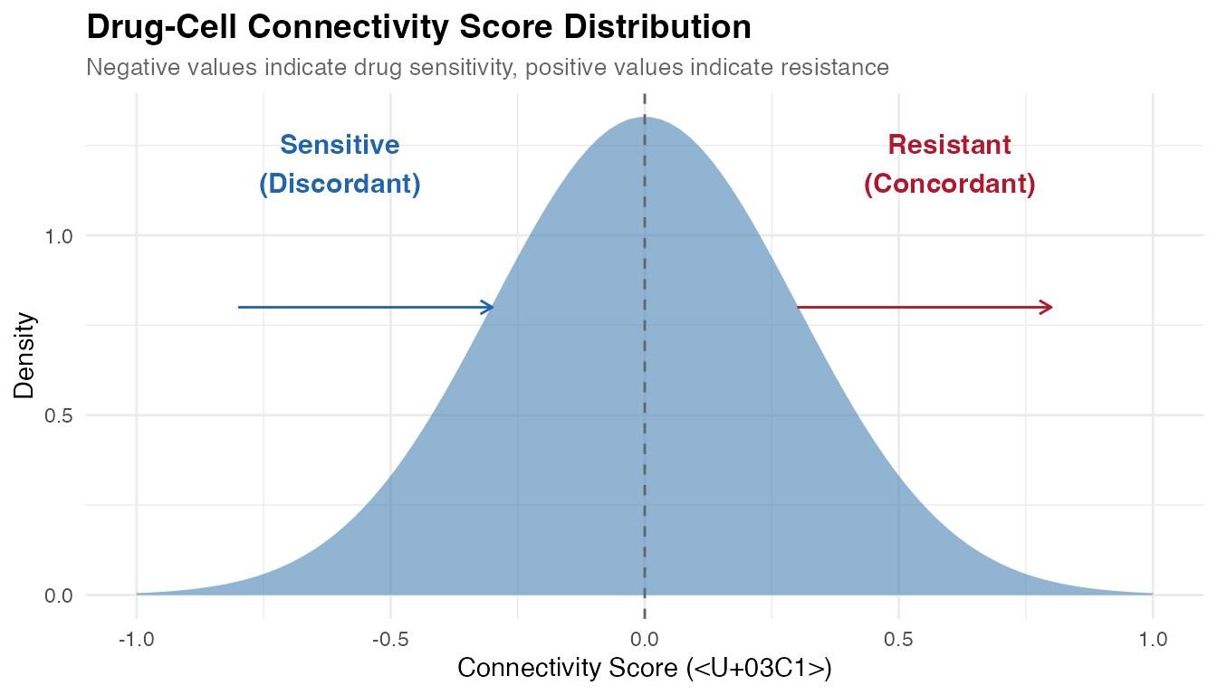
The core innovation of scFOCAL is the Drug-Cell Connectivity Score, which quantifies the transcriptional relationship between individual cells and drug perturbation signatures.

Mathematical Formulation

For each cell $c$ and drug $d$, we compute the Spearman rank correlation:

$$\rho_{c,d} = 1 - \frac{6 \sum_{i=1}^{n} (R_{x_i} - R_{y_i})^2}{n(n^2 - 1)}$$

Where:

• $R_{x_i}$ = rank of gene $i$ expression in cell $c$
• $R_{y_i}$ = rank of gene $i$ in drug signature $d$
• $n$ = number of overlapping genes

Interpretation

Score Range	Interpretation	Biological Meaning
ρ < -0.3	Strong discordance	High drug sensitivity
-0.3 ≤ ρ < 0	Moderate discordance	Moderate sensitivity
0 ≤ ρ < 0.3	Moderate concordance	Moderate resistance
ρ ≥ 0.3	Strong concordance	High drug resistance

2. Fisher’s Z-Transformation

Purpose

To enable statistical comparison of correlation coefficients across conditions, we apply Fisher’s Z-transformation:

$$Z = \frac{1}{2} \ln\left(\frac{1+\rho}{1-\rho}\right) = \text{arctanh}(\rho)$$

Properties

# Demonstrate Fisher Z transformation
rho <- seq(-0.95, 0.95, by = 0.01)
z <- 0.5 * log((1 + rho) / (1 - rho))

df <- data.frame(rho = rho, z = z)

ggplot(df, aes(x = rho, y = z)) +
  geom_line(color = "#0072B2", linewidth = 1.2) +
  geom_hline(yintercept = 0, linetype = "dashed", color = "gray50") +
  geom_vline(xintercept = 0, linetype = "dashed", color = "gray50") +
  labs(
    title = "Fisher's Z-Transformation",
    subtitle = expression(Z == frac(1,2) * ln * bgroup("(", frac(1+rho, 1-rho), ")")),
    x = expression("Correlation coefficient (" * rho * ")"),
    y = "Fisher's Z"
  ) +
  theme_minimal() +
  theme(
    plot.title = element_text(face = "bold", size = 14),
    plot.subtitle = element_text(size = 12)
  )

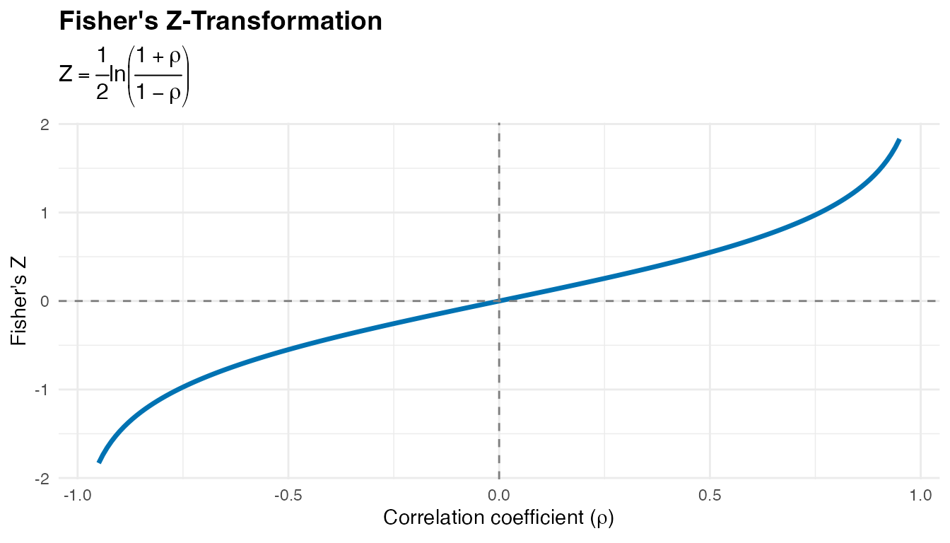
Key advantages:

1. Normalizes the sampling distribution - Z-values follow an approximately normal distribution
2. Stabilizes variance - Variance becomes approximately constant across different correlation values
3. Enables parametric testing - Allows use of standard statistical tests (t-tests, ANOVA)

Variance Property

The variance of Z is approximately:

$$\text{Var}(Z) \approx \frac{1}{n-3}$$

Where $n$ is the number of genes used in correlation.

3. Differential Connectivity Analysis

Linear Model Framework

scFOCAL uses limma (Linear Models for Microarray Data) for differential connectivity analysis:

$$Z_{ij} = \mu + \beta_1 \cdot \text{Subject}_j + \beta_2 \cdot \text{Sensitivity}_i + \epsilon_{ij}$$

Where:

• $Z_{ij}$ = Z-transformed connectivity for cell $i$ in subject $j$
• $\text{Subject}_j$ = blocking factor for subject/replicate
• $\text{Sensitivity}_i$ = binary indicator (sensitive vs resistant)
• $\epsilon_{ij}$ = residual error

Empirical Bayes Moderation

limma applies empirical Bayes moderation to improve variance estimates:

The moderated t-statistic provides:

• Increased statistical power for compounds with few cells
• Robust inference even with small sample sizes
• Proper multiple testing correction via FDR adjustment

4. Disease Signature Reversal Score

Concept

The reversal score quantifies how effectively a drug can reverse disease-associated gene expression changes.

Algorithm

For disease signature $D$ and drug signature $d$:

$$\text{Reversal Score} = \frac{N_{\text{discordant}}}{N_{\text{concordant}}}$$

Where:

• $N_{\text{discordant}}$ = genes where $\text{sign}(D_g) \neq \text{sign}(d_g)$
• $N_{\text{concordant}}$ = genes where $\text{sign}(D_g) = \text{sign}(d_g)$

Interpretation

Reversal Score	Interpretation
> 2.0	Strong reversal potential
1.0 - 2.0	Moderate reversal
< 1.0	Limited reversal

5. MAST Differential Expression

Model Structure

For disease signature computation, scFOCAL employs MAST (Model-based Analysis of Single-cell Transcriptomics):

$$\text{logit}(P(Z_g > 0)) = X\beta_D + W\alpha_D$$

$$E[Y_g | Z_g = 1] = X\beta_C + W\alpha_C$$

Where:

• $Z_g$ = indicator for gene detection
• $Y_g$ = continuous expression level
• $X$ = design matrix (cell type, condition)
• $W$ = cellular detection rate (technical covariate)

Advantages for Single-Cell Data

1. Handles zero-inflation - Explicitly models dropout events
2. Controls for technical variation - Includes cellular detection rate
3. Subject-level effects - Can incorporate random effects for replicates

6. Computational Complexity

Time Complexity Analysis

Operation	Complexity	Typical Runtime
Drug-Cell Connectivity	O(n × m × g)	~20 min for 10K cells
MAST Differential Expression	O(n × g)	~5 min per comparison
Reversal Scoring	O(d × g)	< 1 min
Differential Connectivity	O(n × d)	~2 min

Where: n = cells, m = compounds (1679), g = genes (~1000), d = drug signatures

Memory Requirements

• Minimum: 8 GB RAM
• Recommended: 16 GB RAM for datasets > 50K cells
• Large datasets: Consider chunked processing

Summary

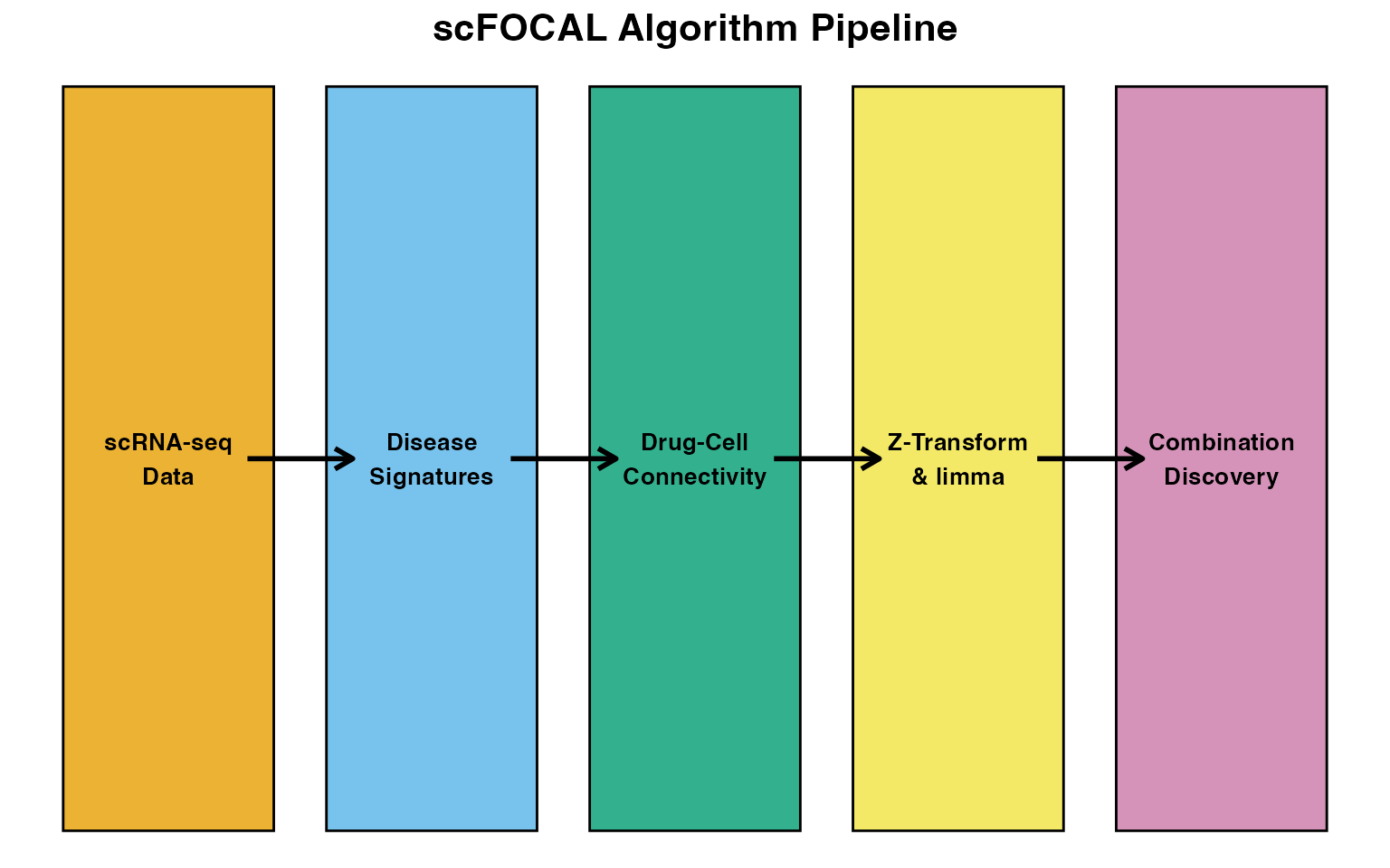
scFOCAL’s algorithmic framework provides:

1. Robust statistical inference through Fisher Z-transformation and empirical Bayes
2. Biological interpretability via connectivity and reversal scores
3. Scalability to large single-cell datasets
4. Integration of orthogonal pharmacological and transcriptomic data

References

1. Subramanian A, et al. A Next Generation Connectivity Map. Cell (2017)
2. Finak G, et al. MAST: a flexible statistical framework. Genome Biology (2015)
3. Ritchie ME, et al. limma powers differential expression. Nucleic Acids Res (2015)
4. Fisher RA. On the probable error of a coefficient of correlation. Metron (1921)

Session Info

sessionInfo()

## R version 4.4.0 (2024-04-24)
## Platform: aarch64-apple-darwin20
## Running under: macOS 15.6.1
## 
## Matrix products: default
## BLAS:   /System/Library/Frameworks/Accelerate.framework/Versions/A/Frameworks/vecLib.framework/Versions/A/libBLAS.dylib 
## LAPACK: /Library/Frameworks/R.framework/Versions/4.4-arm64/Resources/lib/libRlapack.dylib;  LAPACK version 3.12.0
## 
## locale:
## [1] C
## 
## time zone: Asia/Shanghai
## tzcode source: internal
## 
## attached base packages:
## [1] stats     graphics  grDevices utils     datasets  methods   base     
## 
## other attached packages:
## [1] dplyr_1.1.4   ggplot2_4.0.1
## 
## loaded via a namespace (and not attached):
##  [1] gtable_0.3.6       jsonlite_2.0.0     compiler_4.4.0     tidyselect_1.2.1  
##  [5] dichromat_2.0-0.1  jquerylib_0.1.4    systemfonts_1.3.1  scales_1.4.0      
##  [9] textshaping_1.0.4  yaml_2.3.12        fastmap_1.2.0      R6_2.6.1          
## [13] labeling_0.4.3     generics_0.1.4     knitr_1.51         htmlwidgets_1.6.4 
## [17] tibble_3.3.1       desc_1.4.3         bslib_0.9.0        pillar_1.11.1     
## [21] RColorBrewer_1.1-3 rlang_1.1.7        cachem_1.1.0       xfun_0.56         
## [25] fs_1.6.6           sass_0.4.10        S7_0.2.1           otel_0.2.0        
## [29] cli_3.6.5          pkgdown_2.2.0      withr_3.0.2        magrittr_2.0.4    
## [33] digest_0.6.39      grid_4.4.0         lifecycle_1.0.5    vctrs_0.7.1       
## [37] evaluate_1.0.5     glue_1.8.0         farver_2.1.2       ragg_1.5.0        
## [41] rmarkdown_2.30     tools_4.4.0        pkgconfig_2.0.3    htmltools_0.5.9