Algorithm and Methodology

Zaoqu Liu

Department of Interventional Radiology, The First Affiliated Hospital of Zhengzhou University
liuzaoqu@163.com

Aimin Xie

Original Author
aiminyy1993@gmail.com

2026-01-23

Overview

scPAS identifies phenotype-associated cell subpopulations through a multi-step computational pipeline that integrates bulk and single-cell RNA-seq data.

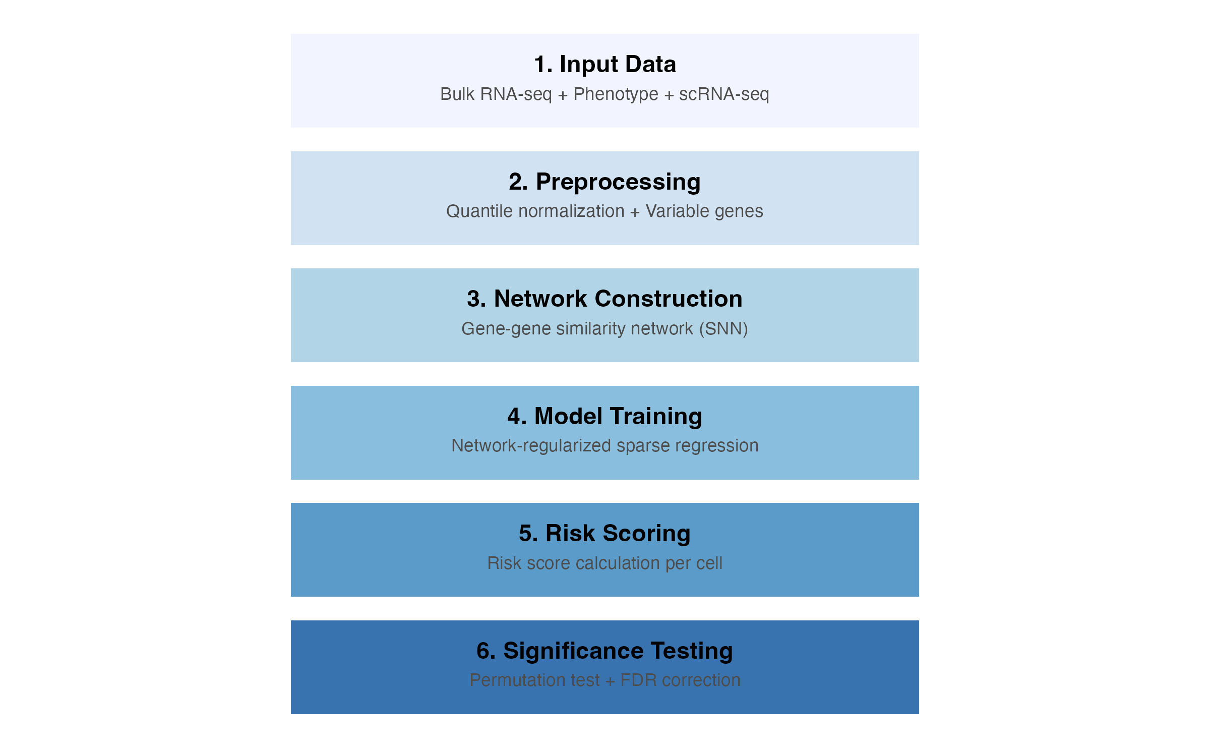
scPAS Workflow Overview

Mathematical Framework

Problem Formulation

Given:

• Bulk expression matrix $\mathbf{X} \in \mathbb{R}^{n \times p}$ (n samples × p genes)
• Phenotype vector $\mathbf{y}$ (continuous, binary, or survival)
• Single-cell expression matrix $\mathbf{S} \in \mathbb{R}^{m \times p}$ (m cells × p genes)

The goal is to find gene weights $\boldsymbol{\beta}$ that associate gene expression with phenotype, then apply these weights to single-cell data to compute per-cell risk scores.

Network-Regularized Sparse Regression

scPAS uses the APML0 (Augmented and Penalized Minimization L0) algorithm with network regularization:

$$\hat{\boldsymbol{\beta}} = \arg\min_{\boldsymbol{\beta}} \left\{ L(\boldsymbol{\beta}; \mathbf{X}, \mathbf{y}) + \lambda_1 \|\boldsymbol{\beta}\|_1 + \lambda_2 \boldsymbol{\beta}^T \mathbf{L} \boldsymbol{\beta} \right\}$$

Where:

• $L(\boldsymbol{\beta})$ is the loss function (depends on phenotype type)
• $\lambda_1 \|\boldsymbol{\beta}\|_1$ is the L1 penalty (LASSO) for sparsity
• $\lambda_2 \boldsymbol{\beta}^T \mathbf{L} \boldsymbol{\beta}$ is the Laplacian penalty for network regularization
• $\mathbf{L}$ is the Laplacian matrix of the gene-gene network

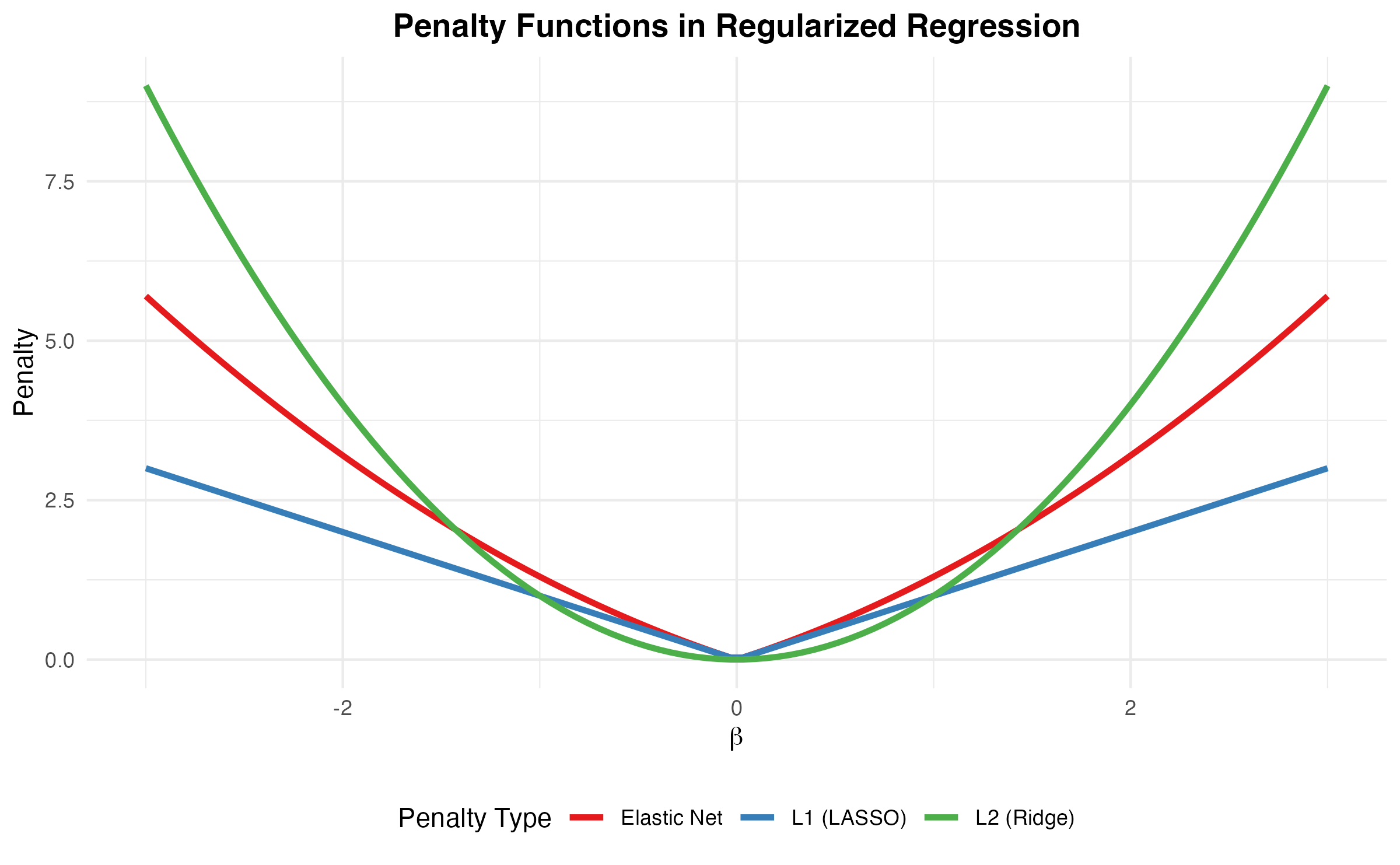
Effect of Network Regularization

Loss Functions by Phenotype Type

Gaussian Family (Continuous)

For continuous phenotypes, we minimize the squared error:

$$L(\boldsymbol{\beta}) = \frac{1}{2n} \sum_{i=1}^{n} (y_i - \mathbf{x}_i^T \boldsymbol{\beta})^2$$

Binomial Family (Binary)

For binary outcomes, we use logistic regression:

$$L(\boldsymbol{\beta}) = -\frac{1}{n} \sum_{i=1}^{n} \left[ y_i \log(p_i) + (1-y_i) \log(1-p_i) \right]$$

where $p_i = \frac{1}{1 + e^{-\mathbf{x}_i^T \boldsymbol{\beta}}}$

Cox Family (Survival)

For time-to-event data, we minimize the negative partial log-likelihood:

$$L(\boldsymbol{\beta}) = -\frac{1}{n} \sum_{i: \delta_i = 1} \left[ \mathbf{x}_i^T \boldsymbol{\beta} - \log \sum_{j \in R(t_i)} e^{\mathbf{x}_j^T \boldsymbol{\beta}} \right]$$

where $R(t_i)$ is the risk set at time $t_i$ and $\delta_i$ is the event indicator.

Gene Network Construction

Shared Nearest Neighbor (SNN) Network

scPAS constructs a gene-gene similarity network from single-cell data using the SNN algorithm:

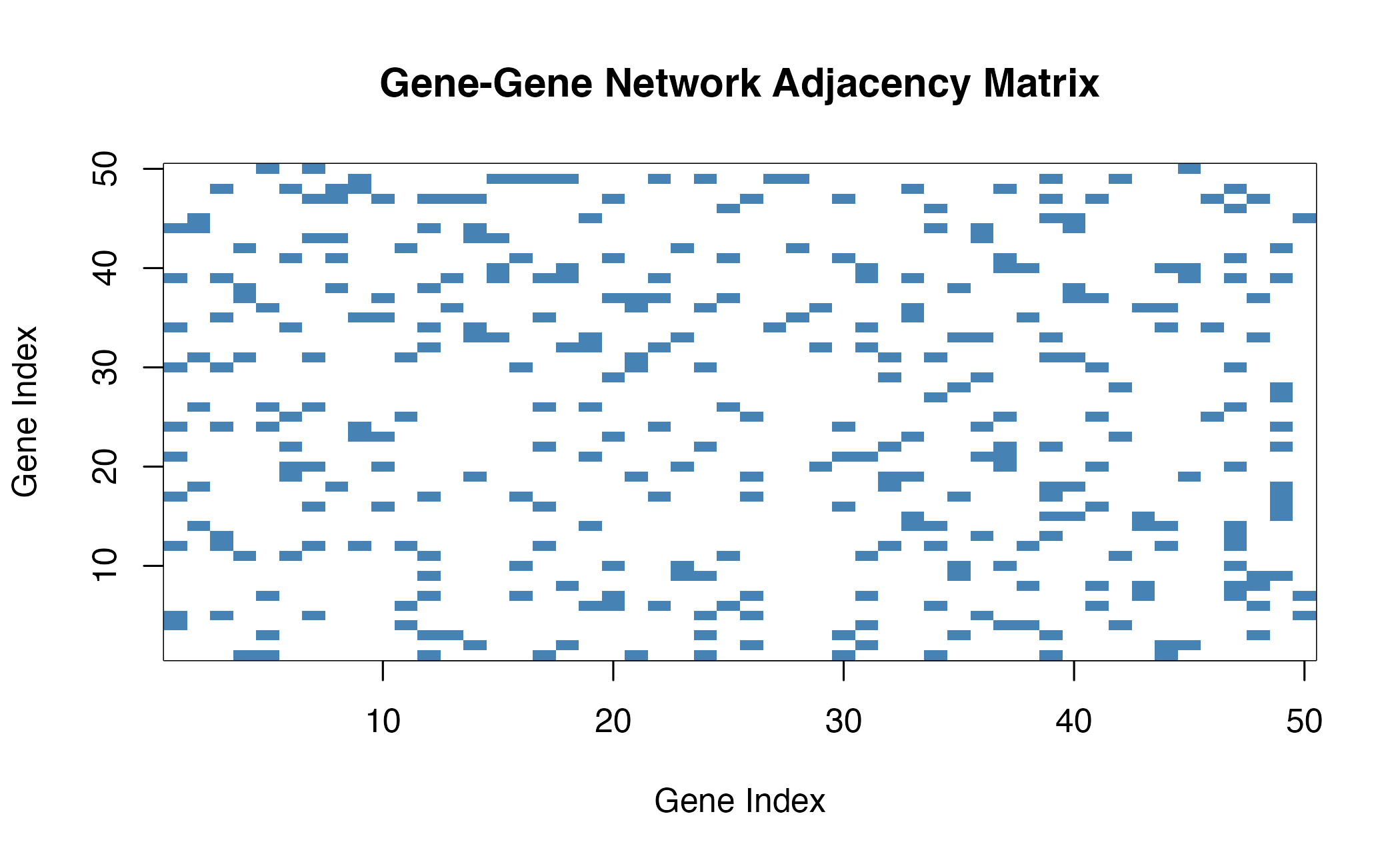
SNN Network Construction

The network construction process:

1. Calculate gene correlations from single-cell expression
2. Find k-nearest neighbors for each gene
3. Compute SNN similarity based on shared neighbors
4. Threshold to create binary adjacency matrix

Risk Score Calculation

Per-Cell Risk Score

Once the model is trained, the risk score for each cell is computed as:

$$RS_j = \sum_{g=1}^{p} \hat{\beta}_g \cdot \tilde{S}_{jg}$$

where:

• $RS_j$ is the risk score for cell $j$
• $\hat{\beta}_g$ is the learned coefficient for gene $g$
• $\tilde{S}_{jg}$ is the standardized expression of gene $g$ in cell $j$

Risk Score Distribution

Normalized Risk Score

The raw risk score is converted to a Z-statistic:

$$NRS_j = \frac{RS_j - \mu_{bg}}{\sigma_{bg}}$$

where $\mu_{bg}$ and $\sigma_{bg}$ are the mean and standard deviation of the background distribution estimated from permutation.

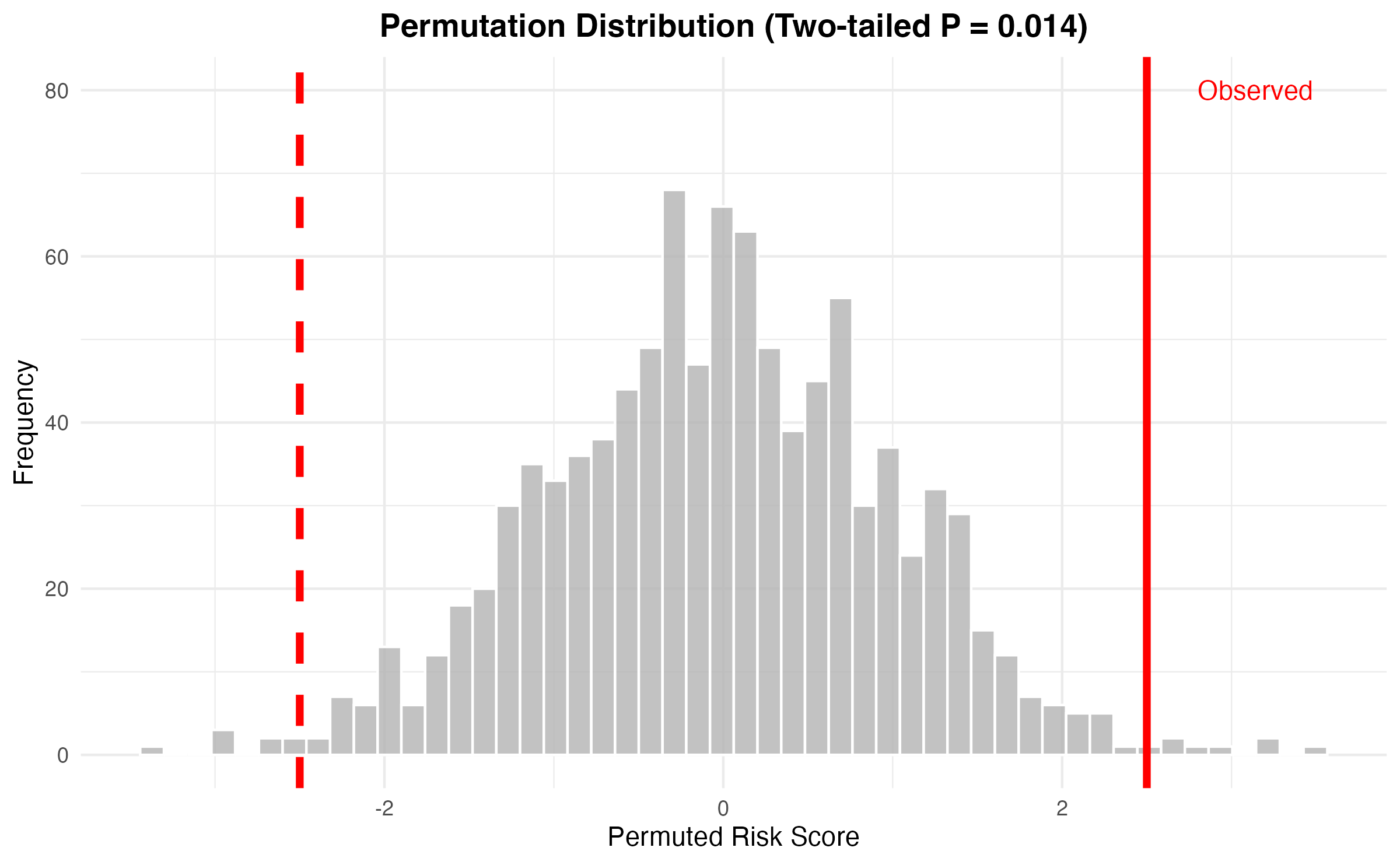
Statistical Significance Testing

Permutation Test

To assess significance, scPAS performs a permutation test:

Permutation Test Principle

Algorithm:

1. For each permutation $b = 1, \ldots, B$:
   • Randomly shuffle the gene coefficients $\boldsymbol{\beta}$
   • Calculate permuted risk scores for all cells
2. Compute two-tailed P-value:

$$p_j = \frac{1}{B} \sum_{b=1}^{B} \mathbb{I}(|RS_j^{(b)}| \geq |RS_j|)$$

FDR Correction

Multiple testing correction using Benjamini-Hochberg procedure:

$$FDR_j = \min\left(1, \frac{p_j \cdot m}{\text{rank}(p_j)}\right)$$

where $m$ is the total number of cells.

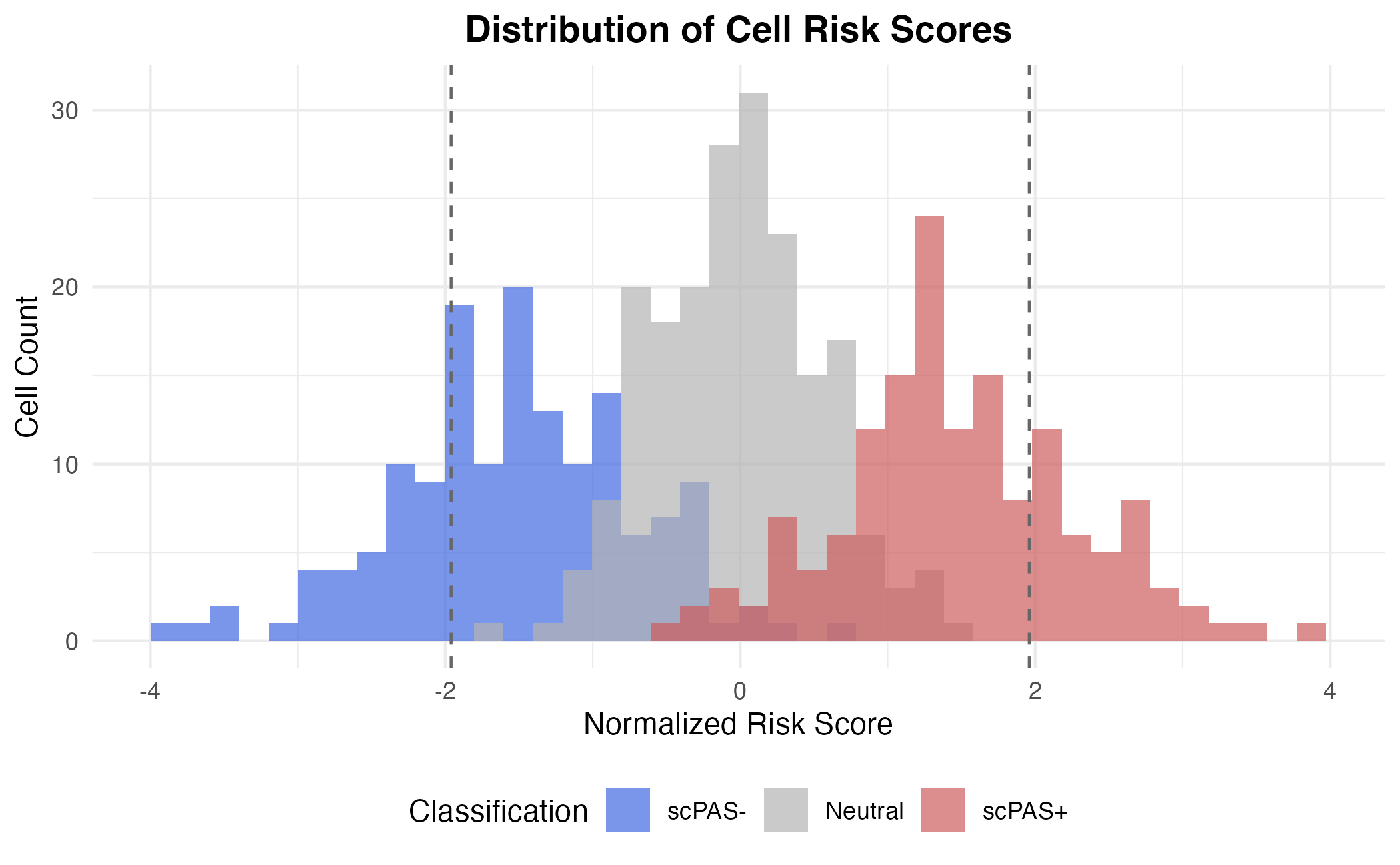
Cell Classification

Cells are classified based on:

1. Statistical significance: FDR < threshold (default 0.05)
2. Direction of association: Sign of normalized risk score

Category	Criteria
scPAS+	FDR < 0.05 AND NRS > 0
scPAS-	FDR < 0.05 AND NRS < 0
0	FDR ≥ 0.05

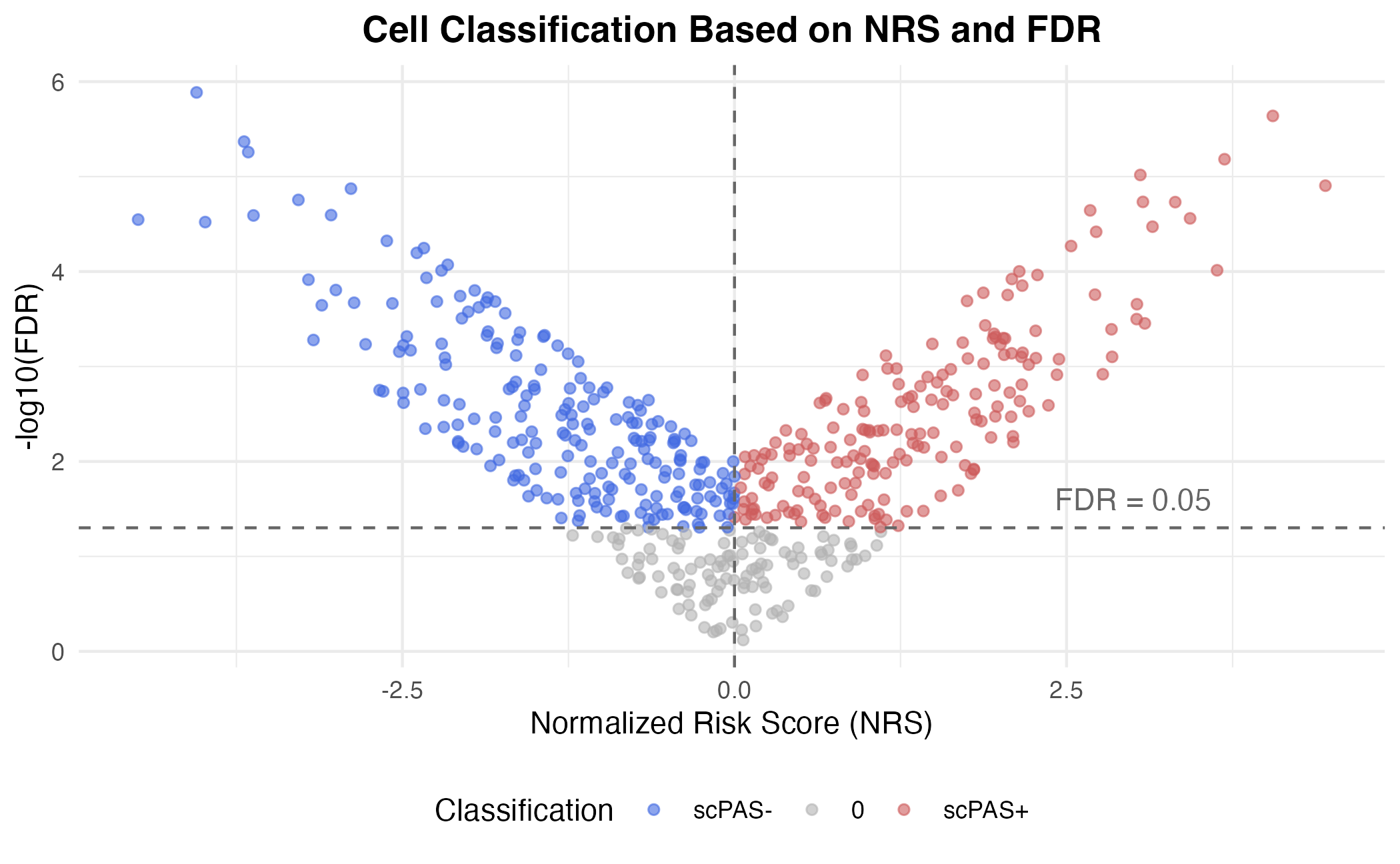
Cell Classification Scheme

Implementation Details

Sparse Matrix Operations

scPAS uses efficient sparse matrix operations for large-scale single-cell data:

# Efficient correlation calculation for sparse matrices
sparse.cor <- function(x) {
  # Uses optimized algorithm that avoids dense conversion
  # Handles numerical precision issues
  # Returns proper correlation matrix
}

# Efficient row scaling
sparse_row_scale <- function(x, center = TRUE, scale = TRUE) {
  # Row-wise standardization
  # Preserves sparsity when only scaling (not centering)
}

Parallel Computing

For large permutation counts, scPAS supports parallel processing:

result <- scPAS(
  bulk_dataset = bulk_data,
  sc_dataset = sc_obj,
  phenotype = phenotype,
  permutation_times = 5000,
  n_cores = 4  # Use 4 CPU cores
)

References

1. Original scPAS Paper: Xie A, et al. (2024). scPAS: single-cell phenotype-associated subpopulation identifier. Briefings in Bioinformatics, 26(1):bbae655.

2. Network-Regularized Regression: Zou H, Hastie T. (2005). Regularization and variable selection via the elastic net. JRSS-B, 67(2):301-320.

3. Permutation Testing: Westfall PH, Young SS. (1993). Resampling-Based Multiple Testing. Wiley.

Session Information

sessionInfo()
#> R version 4.4.0 (2024-04-24)
#> Platform: aarch64-apple-darwin20
#> Running under: macOS 15.6.1
#> 
#> Matrix products: default
#> BLAS:   /Library/Frameworks/R.framework/Versions/4.4-arm64/Resources/lib/libRblas.0.dylib 
#> LAPACK: /Library/Frameworks/R.framework/Versions/4.4-arm64/Resources/lib/libRlapack.dylib;  LAPACK version 3.12.0
#> 
#> locale:
#> [1] C
#> 
#> time zone: Asia/Shanghai
#> tzcode source: internal
#> 
#> attached base packages:
#> [1] stats     graphics  grDevices utils     datasets  methods   base     
#> 
#> other attached packages:
#> [1] Matrix_1.7-4  ggplot2_4.0.1
#> 
#> loaded via a namespace (and not attached):
#>  [1] gtable_0.3.6       jsonlite_2.0.0     dplyr_1.1.4        compiler_4.4.0    
#>  [5] tidyselect_1.2.1   dichromat_2.0-0.1  jquerylib_0.1.4    systemfonts_1.3.1 
#>  [9] scales_1.4.0       textshaping_1.0.4  yaml_2.3.12        fastmap_1.2.0     
#> [13] lattice_0.22-7     R6_2.6.1           labeling_0.4.3     generics_0.1.4    
#> [17] knitr_1.51         htmlwidgets_1.6.4  tibble_3.3.1       desc_1.4.3        
#> [21] bslib_0.9.0        pillar_1.11.1      RColorBrewer_1.1-3 rlang_1.1.7       
#> [25] cachem_1.1.0       xfun_0.56          fs_1.6.6           sass_0.4.10       
#> [29] S7_0.2.1           otel_0.2.0         cli_3.6.5          pkgdown_2.1.3     
#> [33] withr_3.0.2        magrittr_2.0.4     digest_0.6.39      grid_4.4.0        
#> [37] lifecycle_1.0.5    vctrs_0.7.0        evaluate_1.0.5     glue_1.8.0        
#> [41] farver_2.1.2       ragg_1.5.0         rmarkdown_2.30     tools_4.4.0       
#> [45] pkgconfig_2.0.3    htmltools_0.5.9