Algorithm Theory and Mathematical Foundation

Overview

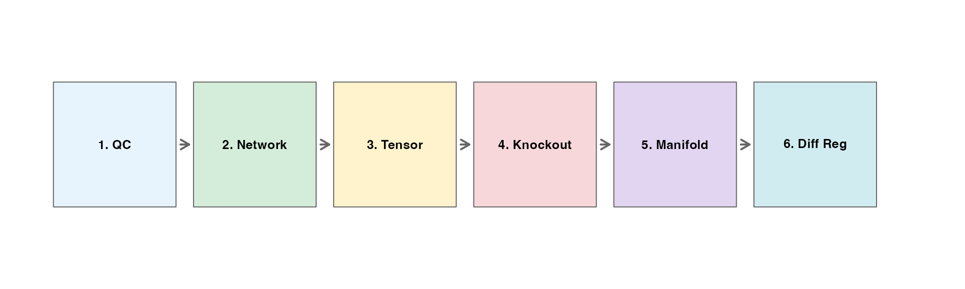
The scTenifoldKnk workflow consists of six main steps:

Quality Control - Filter cells and genes
Network Construction - Build gene regulatory networks using PCR
Tensor Decomposition - Denoise networks via CP decomposition
Virtual Knockout - Simulate gene knockout
Manifold Alignment - Align WT and KO networks
Differential Regulation - Identify affected genes

Step 1: Quality Control

Mathematical Formulation

Let $X \in \mathbb{R}^{G \times C}$ be the count matrix where $G$ is the number of genes and $C$ is the number of cells.

Library Size Filter: $L_j = \sum_{i=1}^{G} X_{ij}, \quad \text{keep cell } j \text{ if } L_j \geq L_{min}$

Gene Detection Filter: $D_i = \sum_{j=1}^{C} \mathbb{1}(X_{ij} > 0), \quad \text{keep gene } i \text{ if } D_i \geq D_{min}$

Mitochondrial Content Filter: $MT_j = \frac{\sum_{i \in MT} X_{ij}}{L_j}, \quad \text{keep cell } j \text{ if } MT_j \leq MT_{max}$

library(scTenifoldKnk)

# Load data
data_path <- system.file("single-cell/example.csv", package = "scTenifoldKnk")
scRNAseq <- as.matrix(read.csv(data_path, row.names = 1))

# Compute library sizes
library_sizes <- colSums(scRNAseq)

# Visualize library size distribution
hist(library_sizes, breaks = 30, col = "#4A90D9", border = "white",
     main = "Library Size Distribution",
     xlab = "Total UMI counts per cell")
abline(v = 1000, col = "red", lwd = 2, lty = 2)
legend("topright", "Threshold = 1000", col = "red", lty = 2, lwd = 2, bty = "n")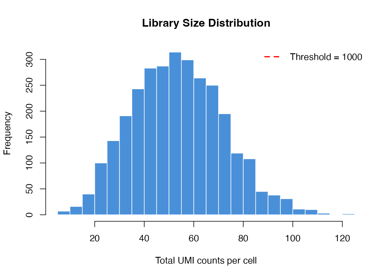

Step 2: Network Construction (Principal Component Regression)

Algorithm

For each gene $k$ , we perform leave-one-out principal component regression:

Center and scale the expression matrix $X$
Exclude gene $k$ : $X_{-k} \in \mathbb{R}^{C \times (G-1)}$
Compute SVD: $X_{-k} = U \Sigma V^T$
Extract top $p$ components: $PC = U_p \Sigma_p$
Regress gene $k$ on PCs: $\beta = (PC^T PC)^{-1} PC^T y_k$
Transform back: $W_{k,-k} = V_p \beta$

Mathematical Derivation

The network weight $W_{ij}$ represents the regulatory relationship:

$W_{ij} = \text{Cov}(X_i, X_j | PC_{-i})$

This captures the conditional covariance between genes through the principal component space.

# Illustrate PCA on gene expression
set.seed(42)
X <- matrix(rpois(500, 10), nrow = 50, ncol = 10)
rownames(X) <- paste0("Gene", 1:50)
X <- X[rowSums(X) > 0, ]

# Standardize
X_scaled <- scale(t(X))

# PCA
pca <- prcomp(X_scaled, center = FALSE)

# Visualize
par(mfrow = c(1, 2))

# PC scores
plot(pca$x[, 1], pca$x[, 2],
     pch = 19, col = "#4A90D9",
     xlab = "PC1", ylab = "PC2",
     main = "Cell Embeddings (PC Space)")

# Variance explained
var_explained <- (pca$sdev^2 / sum(pca$sdev^2)) * 100
barplot(var_explained[1:10], 
        names.arg = paste0("PC", 1:10),
        col = "#4A90D9",
        main = "Variance Explained",
        ylab = "% Variance",
        las = 2)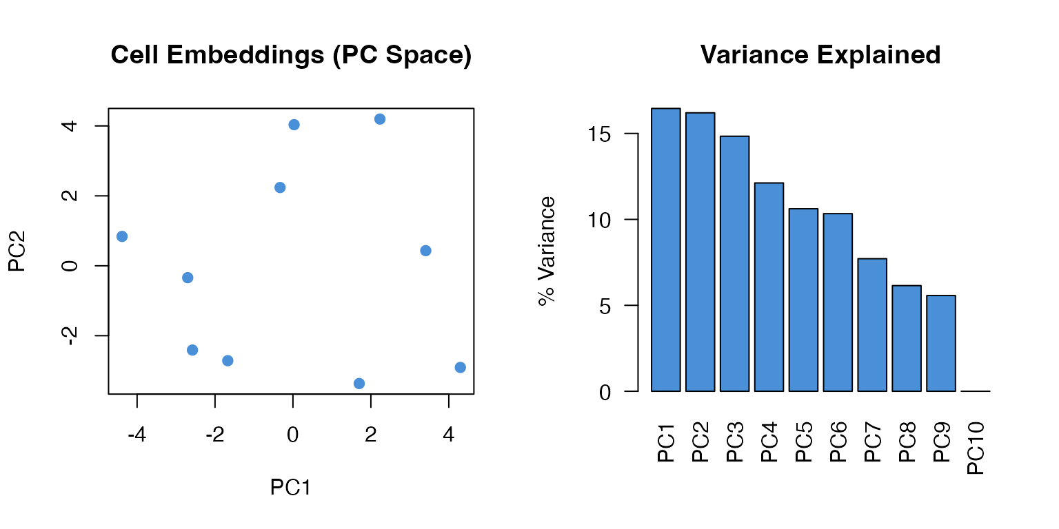

Step 3: Tensor Decomposition (CP-ALS)

CANDECOMP/PARAFAC Decomposition

Given a 3-way tensor $\mathcal{X} \in \mathbb{R}^{G \times G \times N}$ (networks stacked along third mode):

$\mathcal{X} \approx \sum_{r=1}^{R} \lambda_r \cdot a_r \otimes b_r \otimes c_r$

where: - $a_r, b_r \in \mathbb{R}^G$ are gene factor vectors - $c_r \in \mathbb{R}^N$ are network weights - $\lambda_r$ are component weights - $\otimes$ denotes outer product

Alternating Least Squares (ALS) Algorithm

For each mode $n \in \{1, 2, 3\}$ :

$A^{(n)} \leftarrow X_{(n)} (A^{(-n)})^{\dagger}$

where $X_{(n)}$ is the mode- $n$ unfolding and $(A^{(-n)})^{\dagger}$ is the Khatri-Rao product pseudoinverse.

Reconstruction

The denoised network is the weighted average:

$\bar{W} = \frac{1}{N} \sum_{k=1}^{N} \sum_{r=1}^{R} c_{kr} \cdot a_r b_r^T$

# Build multiple networks
networks <- makeNetworksFast(X, nNet = 5, nCells = 8, nComp = 3, 
                              verbose = FALSE, seed = 42)

# Tensor decomposition
td_result <- tensorDecomposition(networks, K = 3, maxIter = 100)

# Visualize reconstruction
par(mfrow = c(1, 2))

# Original (first network)
net1 <- as.matrix(networks[[1]])
image(net1[1:20, 1:20], 
      col = colorRampPalette(c("blue", "white", "red"))(100),
      main = "Original Network (slice 1)",
      xlab = "Genes", ylab = "Genes", axes = FALSE)

# Reconstructed
recon <- as.matrix(td_result$X)
image(recon[1:20, 1:20],
      col = colorRampPalette(c("blue", "white", "red"))(100),
      main = "Reconstructed (Denoised)",
      xlab = "Genes", ylab = "Genes", axes = FALSE)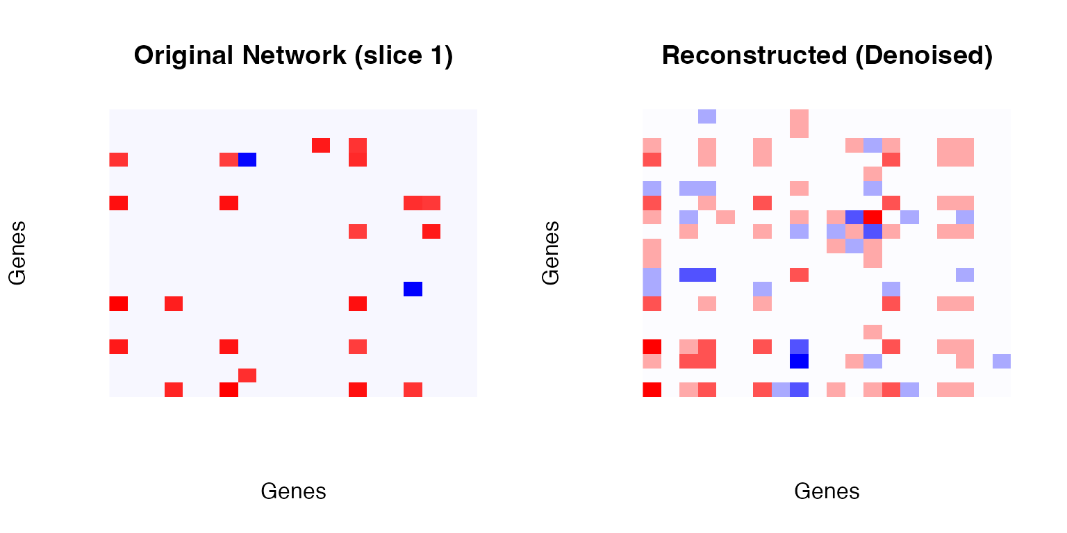

Step 4: Virtual Knockout

Implementation

The knockout operation sets all outgoing edges from gene $g$ to zero:

$W^{KO}_{g, \cdot} = 0$

This simulates the loss of regulatory capacity of gene $g$ .

# Get WT network
WT <- as.matrix(td_result$X)

# Perform knockout
KO <- WT
knockout_gene <- "Gene1"
if (knockout_gene %in% rownames(KO)) {
  ko_idx <- which(rownames(KO) == knockout_gene)
  KO[ko_idx, ] <- 0
}

# Visualize difference
par(mfrow = c(1, 3))

# WT
image(WT[1:15, 1:15],
      col = colorRampPalette(c("blue", "white", "red"))(100),
      main = "Wild-Type Network",
      axes = FALSE)

# KO
image(KO[1:15, 1:15],
      col = colorRampPalette(c("blue", "white", "red"))(100),
      main = paste("Knockout:", knockout_gene),
      axes = FALSE)

# Difference
diff_net <- WT - KO
image(diff_net[1:15, 1:15],
      col = colorRampPalette(c("purple", "white", "orange"))(100),
      main = "Difference (WT - KO)",
      axes = FALSE)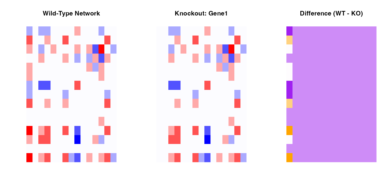

Step 5: Manifold Alignment

Non-linear Manifold Alignment (NLMA)

Given two networks $W^{WT}$ and $W^{KO}$ , we construct a joint graph:

$W = \begin{pmatrix} W^{WT} + I & \mu L \\ \mu L^T & W^{KO} + I \end{pmatrix}$

where $L$ is the alignment matrix and $\mu$ controls alignment strength.

Spectral Embedding

Compute the graph Laplacian: $\mathcal{L} = D - W$

where $D_{ii} = \sum_j W_{ij}$ .

The embedding is given by the eigenvectors corresponding to the smallest non-zero eigenvalues.

# Perform manifold alignment
MA <- manifoldAlignment(Matrix::Matrix(WT, sparse = TRUE), 
                        Matrix::Matrix(KO, sparse = TRUE), 
                        d = 2)

# Extract WT and KO embeddings
n_genes <- nrow(WT)
WT_embed <- MA[1:n_genes, ]
KO_embed <- MA[(n_genes+1):(2*n_genes), ]

# Compute distances
distances <- sqrt(rowSums((WT_embed - KO_embed)^2))

# Plot
plot(WT_embed[, 1], WT_embed[, 2],
     pch = 19, col = "#4A90D9", cex = 0.8,
     xlab = "NLMA Dimension 1", ylab = "NLMA Dimension 2",
     main = "Manifold Alignment Visualization")
points(KO_embed[, 1], KO_embed[, 2],
       pch = 17, col = "#D94A4A", cex = 0.8)

# Draw connections for top affected genes
top_idx <- order(distances, decreasing = TRUE)[1:5]
for (i in top_idx) {
  lines(c(WT_embed[i, 1], KO_embed[i, 1]),
        c(WT_embed[i, 2], KO_embed[i, 2]),
        col = "orange", lwd = 2)
}

legend("topright", 
       legend = c("WT genes", "KO genes", "Top affected"),
       col = c("#4A90D9", "#D94A4A", "orange"),
       pch = c(19, 17, NA), lty = c(NA, NA, 1), lwd = c(NA, NA, 2),
       bty = "n")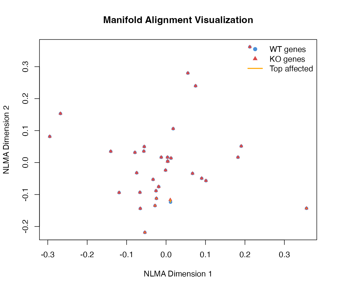

Step 6: Differential Regulation Analysis

Distance-Based Statistics

For each gene $i$ , compute the Euclidean distance between WT and KO embeddings:

$d_i = \|E^{WT}_i - E^{KO}_i\|_2$

Fold Change

$FC_i = \frac{d_i^2}{\bar{d}_{-g}^2}$

where $\bar{d}_{-g}^2 = \frac{1}{G-1}\sum_{j \neq g} d_j^2$ excludes the knockout gene.

Statistical Testing

Under the null hypothesis, $FC$ follows a chi-square distribution:

$FC \sim \chi^2_1$

P-values are computed as: $p_i = P(\chi^2_1 > FC_i)$

Multiple Testing Correction

Benjamini-Hochberg FDR: $p_{adj}^{(i)} = \min\left(1, \frac{n \cdot p_{(i)}}{i}\right)$

# Compute statistics
names(distances) <- rownames(WT)

# Box-Cox transformation
distances_pos <- pmax(distances, 1e-10)
bc_result <- MASS::boxcox(distances_pos ~ 1, plotit = FALSE)
lambda_opt <- bc_result$x[which.max(bc_result$y)]

# Apply transformation
if (abs(lambda_opt) < 0.01) {
  transformed <- log(distances_pos)
} else {
  transformed <- distances_pos^lambda_opt
}

# Z-scores
Z <- scale(transformed)[, 1]

par(mfrow = c(1, 2))

# Box-Cox optimization
plot(bc_result$x, bc_result$y, type = "l", lwd = 2,
     xlab = expression(lambda), ylab = "Log-Likelihood",
     main = "Box-Cox Transformation")
abline(v = lambda_opt, col = "red", lty = 2)
legend("topright", paste("Optimal λ =", round(lambda_opt, 2)),
       col = "red", lty = 2, bty = "n")

# Q-Q plot
qqnorm(Z, main = "Q-Q Plot (After Transformation)", pch = 19, col = "#4A90D9")
qqline(Z, col = "red", lwd = 2)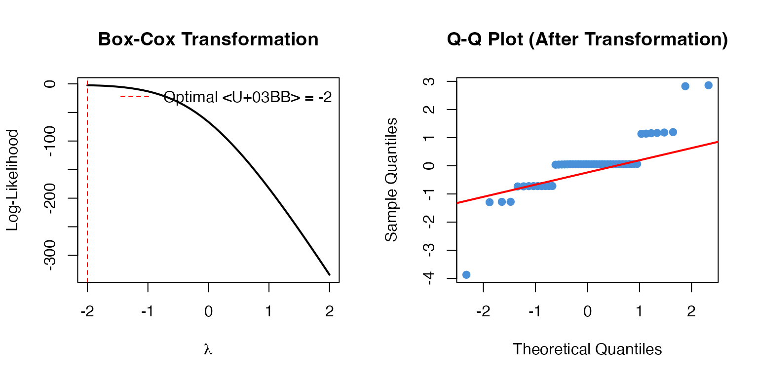

Summary

The scTenifoldKnk algorithm provides a mathematically rigorous framework for:

Network inference via principal component regression
Noise reduction via tensor decomposition
Comparative analysis via manifold alignment
Statistical testing via chi-square distribution

This enables researchers to predict gene knockout effects in silico, saving time and resources compared to wet-lab experiments.

References

Osorio, D., et al. (2020). scTenifoldKnk: An efficient virtual knockout tool for gene function predictions via single-cell gene regulatory network perturbation.
Kolda, T. G., & Bader, B. W. (2009). Tensor decompositions and applications. SIAM review.
Box, G. E., & Cox, D. R. (1964). An analysis of transformations. Journal of the Royal Statistical Society.

Session Info

sessionInfo()
#> R version 4.4.0 (2024-04-24)
#> Platform: aarch64-apple-darwin20
#> Running under: macOS 15.6.1
#> 
#> Matrix products: default
#> BLAS:   /Library/Frameworks/R.framework/Versions/4.4-arm64/Resources/lib/libRblas.0.dylib 
#> LAPACK: /Library/Frameworks/R.framework/Versions/4.4-arm64/Resources/lib/libRlapack.dylib;  LAPACK version 3.12.0
#> 
#> locale:
#> [1] C
#> 
#> time zone: Asia/Shanghai
#> tzcode source: internal
#> 
#> attached base packages:
#> [1] stats     graphics  grDevices utils     datasets  methods   base     
#> 
#> other attached packages:
#> [1] scTenifoldKnk_2.1.0
#> 
#> loaded via a namespace (and not attached):
#>  [1] cli_3.6.5         knitr_1.51        rlang_1.1.7       xfun_0.56        
#>  [5] otel_0.2.0        textshaping_1.0.4 jsonlite_2.0.0    htmltools_0.5.9  
#>  [9] ragg_1.5.0        sass_0.4.10       rmarkdown_2.30    grid_4.4.0       
#> [13] evaluate_1.0.5    jquerylib_0.1.4   MASS_7.3-65       fastmap_1.2.0    
#> [17] yaml_2.3.12       lifecycle_1.0.5   compiler_4.4.0    RSpectra_0.16-2  
#> [21] fs_1.6.6          htmlwidgets_1.6.4 Rcpp_1.1.1        lattice_0.22-7   
#> [25] systemfonts_1.3.1 digest_0.6.39     R6_2.6.1          parallel_4.4.0   
#> [29] bslib_0.9.0       Matrix_1.7-4      tools_4.4.0       pkgdown_2.1.3    
#> [33] cachem_1.1.0      desc_1.4.3

Zaoqu Liu

2026-01-23