Result Interpretation Guide

Introduction

This guide helps you interpret the results from scTenifoldKnk analysis. Understanding what each output component means is crucial for biological interpretation.

Run Analysis

library(scTenifoldKnk)
library(Matrix)

data_path <- system.file("single-cell/example.csv", package = "scTenifoldKnk")
scRNAseq <- as.matrix(read.csv(data_path, row.names = 1))

result <- scTenifoldKnk(
  countMatrix = scRNAseq,
  gKO = "G100",
  qc_minLSize = 0,
  nc_nNet = 5,
  nc_nCells = 100,
  verbose = FALSE
)

Output Structure

# View output structure
str(result, max.level = 2)
#> List of 3
#>  $ tensorNetworks   :List of 2
#>   ..$ WT:Formal class 'dgCMatrix' [package "Matrix"] with 6 slots
#>   ..$ KO:Formal class 'dgCMatrix' [package "Matrix"] with 6 slots
#>  $ manifoldAlignment: num [1:200, 1:2] -0.000319 -0.001996 -0.003614 -0.001457 -0.010918 ...
#>   ..- attr(*, "dimnames")=List of 2
#>  $ diffRegulation   :'data.frame':   100 obs. of  6 variables:
#>   ..$ gene    : chr [1:100] "G100" "G31" "G29" "G24" ...
#>   ..$ distance: num [1:100] 4.99e-04 5.72e-06 5.68e-06 5.67e-06 5.66e-06 ...
#>   ..$ Z       : num [1:100] -8.467 -0.94 -0.847 -0.821 -0.791 ...
#>   ..$ FC      : num [1:100] 8629.87 1.13 1.12 1.11 1.11 ...
#>   ..$ p.value : num [1:100] 0 0.287 0.29 0.291 0.292 ...
#>   ..$ p.adj   : num [1:100] 0 0.346 0.346 0.346 0.346 ...

The output contains four main components:

tensorNetworks$WT: Wild-type gene regulatory network
tensorNetworks$KO: Knockout gene regulatory network
manifoldAlignment: Low-dimensional embedding of genes
diffRegulation: Differential regulation statistics

Understanding the Differential Regulation Table

dr <- result$diffRegulation
knitr::kable(head(dr, 10), digits = 4,
             caption = "Top 10 Differentially Regulated Genes")

Top 10 Differentially Regulated Genes
	gene	distance	Z	FC	p.value	p.adj
G100	G100	5e-04	-8.4673	8629.8672	0.0000	0.0000
G31	G31	0e+00	-0.9401	1.1321	0.2873	0.3455
G29	G29	0e+00	-0.8468	1.1182	0.2903	0.3455
G24	G24	0e+00	-0.8212	1.1145	0.2911	0.3455
G38	G38	0e+00	-0.7912	1.1101	0.2921	0.3455
G39	G39	0e+00	-0.7849	1.1092	0.2923	0.3455
G23	G23	0e+00	-0.7263	1.1008	0.2941	0.3455
G18	G18	0e+00	-0.7072	1.0981	0.2947	0.3455
G19	G19	0e+00	-0.6893	1.0956	0.2952	0.3455
G34	G34	0e+00	-0.6667	1.0924	0.2959	0.3455

Column Descriptions

Column	Description	Interpretation
gene	Gene name	Gene identifier
distance	Euclidean distance	Higher = more affected by knockout
Z	Z-score	Standardized distance
FC	Fold Change	Ratio of gene’s impact to background
p.value	Raw p-value	Statistical significance
p.adj	Adjusted p-value	FDR-corrected significance

Key Metrics Explained

Distance

The distance measures how much a gene’s regulatory profile changes after knockout:

par(mfrow = c(1, 2))

# Distance distribution
hist(dr$distance, breaks = 30, col = "#3498DB", border = "white",
     main = "Distance Distribution",
     xlab = "Euclidean Distance")

# Highlight knockout gene
ko_dist <- dr$distance[dr$gene == "G100"]
abline(v = ko_dist, col = "red", lwd = 2)
text(ko_dist, par("usr")[4] * 0.9, "G100", pos = 4, col = "red")

# Distance vs Rank
plot(1:nrow(dr), dr$distance,
     pch = 19, col = "#3498DB", cex = 0.6,
     xlab = "Rank", ylab = "Distance",
     main = "Distance by Rank")
points(which(dr$gene == "G100"), ko_dist, pch = 17, col = "red", cex = 2)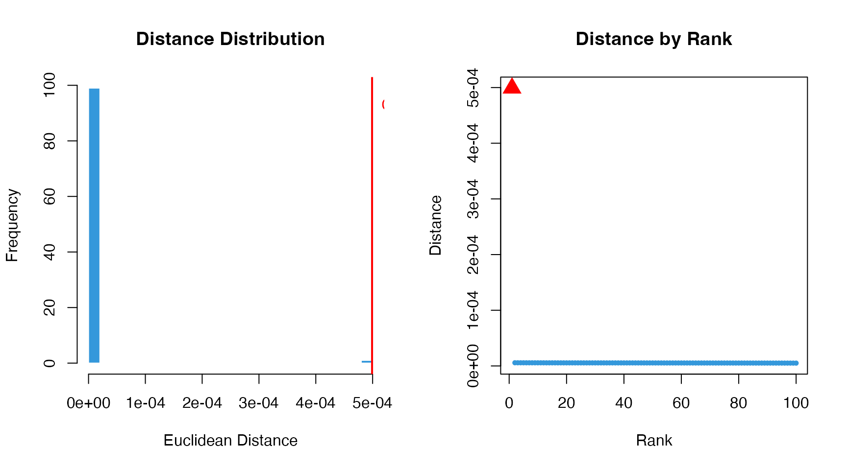

Interpretation: - The knockout gene (G100) should have the highest distance - Genes with high distances are most affected by the knockout - These may be direct targets or closely connected in the network

Fold Change (FC)

FC measures how unusual a gene’s distance is compared to the background:

$FC_i = \frac{d_i^2}{\bar{d}_{-KO}^2}$

# FC distribution
par(mar = c(5, 5, 4, 2))
plot(dr$distance, dr$FC,
     pch = 19, col = "#3498DB", cex = 0.8,
     xlab = "Distance", ylab = "Fold Change",
     main = "Relationship: Distance vs Fold Change")

# The knockout gene
points(dr$distance[dr$gene == "G100"], dr$FC[dr$gene == "G100"],
       pch = 17, col = "red", cex = 2)

# Add trend
fit <- lm(FC ~ poly(distance, 2), data = dr)
x_seq <- seq(min(dr$distance), max(dr$distance), length.out = 100)
lines(x_seq, predict(fit, data.frame(distance = x_seq)), 
      col = "#E74C3C", lwd = 2)

legend("topleft", c("All genes", "G100 (KO)", "Trend"),
       pch = c(19, 17, NA), lty = c(NA, NA, 1),
       col = c("#3498DB", "red", "#E74C3C"), bty = "n")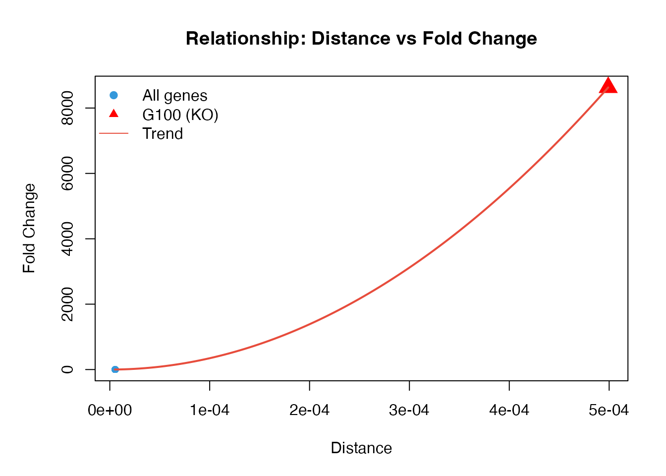

Interpretation: - FC > 1: Gene is more affected than average - FC >> 1: Gene is strongly affected - The knockout gene typically has the highest FC

Statistical Significance

P-values are calculated using chi-square distribution:

par(mfrow = c(1, 2))

# P-value vs FC
plot(dr$FC, -log10(dr$p.value + 1e-300),
     pch = 19, col = "#3498DB", cex = 0.8,
     xlab = "Fold Change", ylab = "-log10(p-value)",
     main = "FC vs Statistical Significance")
abline(h = -log10(0.05), lty = 2, col = "gray40")

# Q-Q plot for chi-square
theoretical <- qchisq(ppoints(nrow(dr)), df = 1)
observed <- sort(dr$FC)

plot(theoretical, observed,
     pch = 19, col = "#3498DB", cex = 0.6,
     xlab = expression(Theoretical~chi[1]^2),
     ylab = "Observed FC",
     main = "Chi-square Q-Q Plot")
abline(0, 1, col = "red", lwd = 2)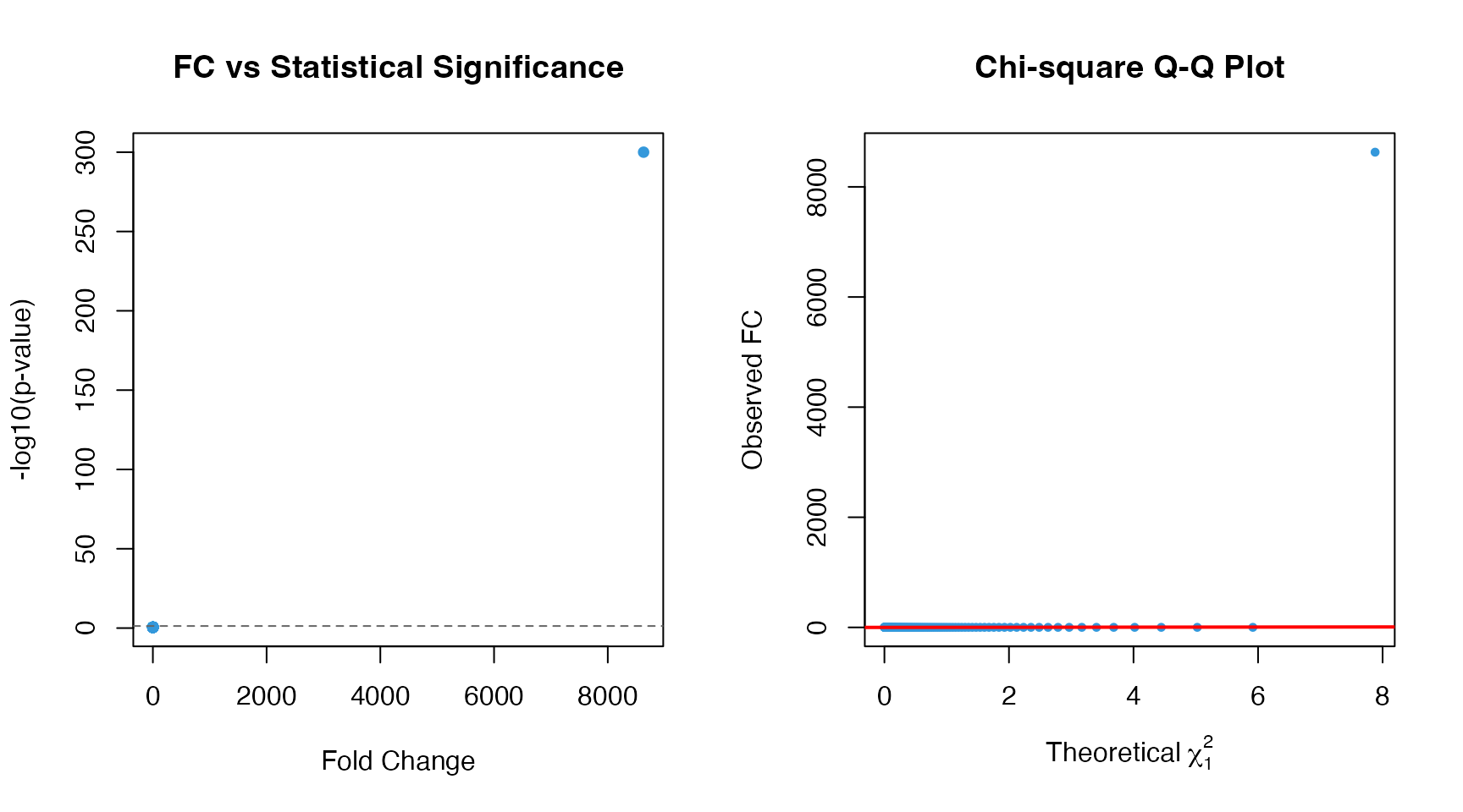

Interpreting the Gene Regulatory Networks

Network Comparison

WT <- as.matrix(result$tensorNetworks$WT)
KO <- as.matrix(result$tensorNetworks$KO)

# Focus on top affected genes
top_genes <- head(dr$gene, 10)

par(mfrow = c(1, 2))

# WT network subset
WT_sub <- WT[top_genes, top_genes]
image(1:10, 1:10, WT_sub,
      col = colorRampPalette(c("blue", "white", "red"))(100),
      axes = FALSE, main = "WT Network (Top 10 Genes)",
      xlab = "", ylab = "")
axis(1, 1:10, top_genes, las = 2, cex.axis = 0.7)
axis(2, 1:10, top_genes, las = 2, cex.axis = 0.7)

# KO network subset
KO_sub <- KO[top_genes, top_genes]
image(1:10, 1:10, KO_sub,
      col = colorRampPalette(c("blue", "white", "red"))(100),
      axes = FALSE, main = "KO Network (Top 10 Genes)",
      xlab = "", ylab = "")
axis(1, 1:10, top_genes, las = 2, cex.axis = 0.7)
axis(2, 1:10, top_genes, las = 2, cex.axis = 0.7)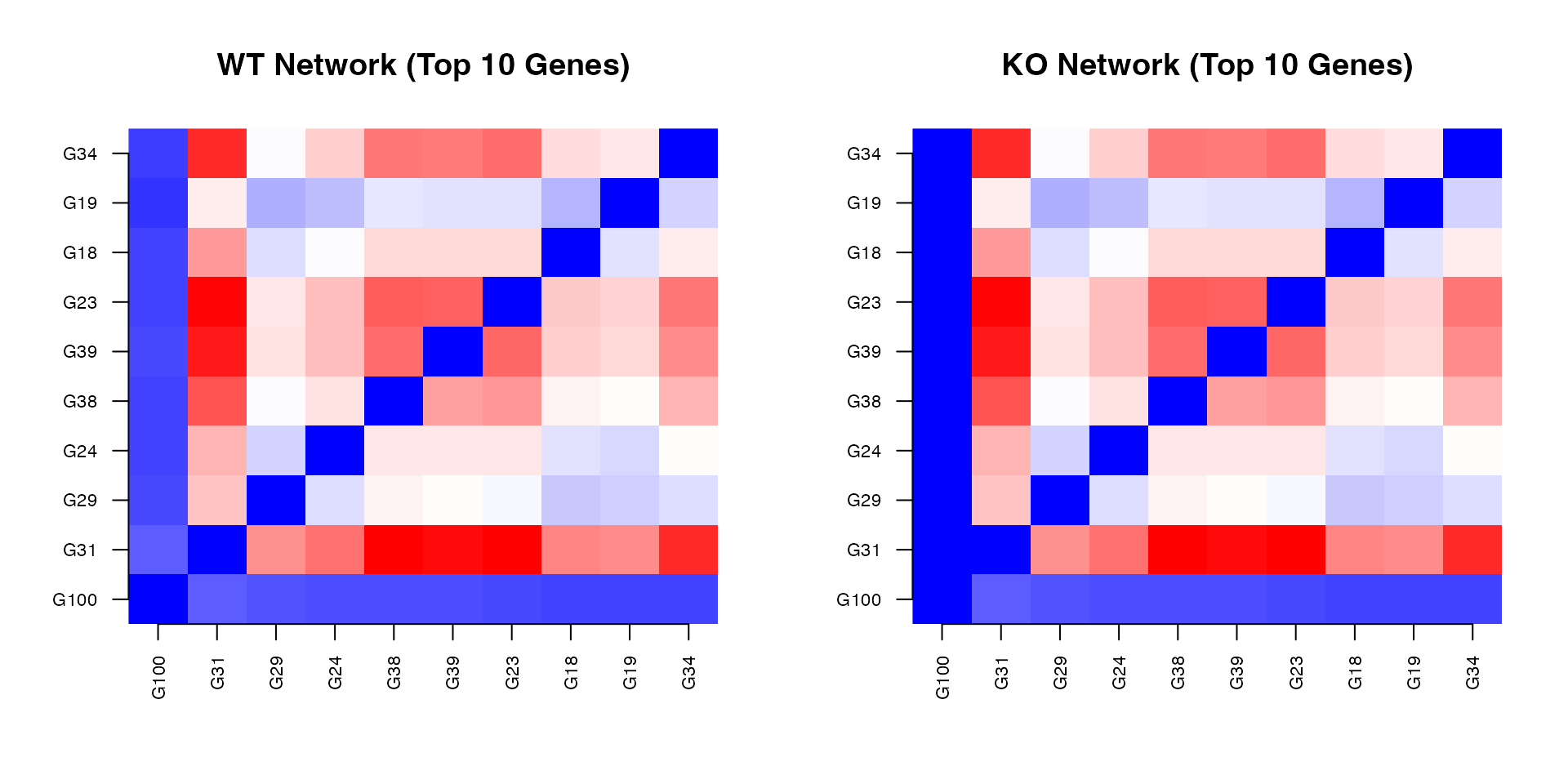

Knockout Effect on Network

# Compute network changes
diff_net <- WT - KO

# For knockout gene
ko_gene <- "G100"
if (ko_gene %in% rownames(WT)) {
  # Outgoing edges (regulatory targets)
  out_edges_WT <- WT[ko_gene, ]
  out_edges_KO <- KO[ko_gene, ]
  
  # Visualize
  par(mar = c(5, 5, 4, 2))
  
  plot(out_edges_WT, type = "h", col = "#3498DB", lwd = 2,
       ylim = range(c(out_edges_WT, out_edges_KO)),
       xlab = "Target Gene Index", ylab = "Edge Weight",
       main = paste("Outgoing Edges from", ko_gene))
  points(1:length(out_edges_KO), out_edges_KO, 
         type = "h", col = "#E74C3C", lwd = 2)
  
  legend("topright", c("WT", "KO"), col = c("#3498DB", "#E74C3C"),
         lwd = 2, bty = "n")
  
  cat("Sum of WT outgoing edges:", round(sum(abs(out_edges_WT)), 4), "\n")
  cat("Sum of KO outgoing edges:", round(sum(abs(out_edges_KO)), 4), "\n")
}

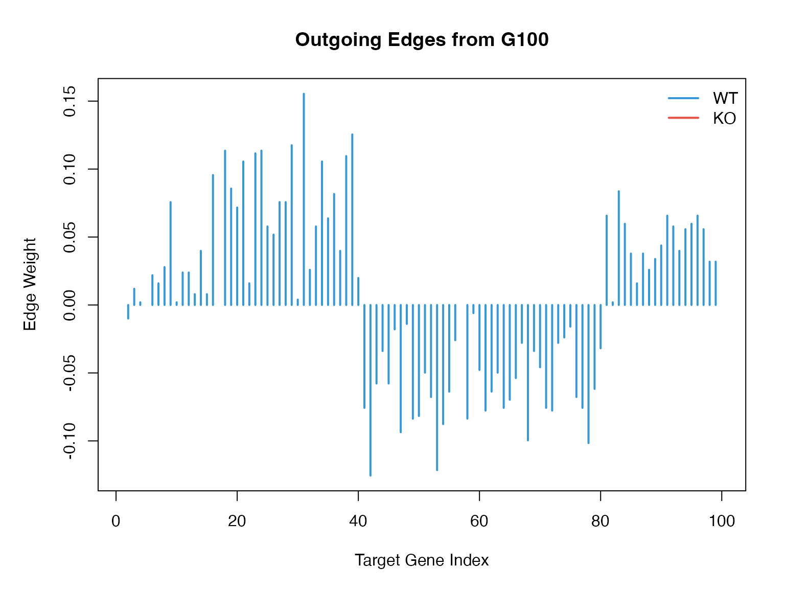
#> Sum of WT outgoing edges: 5.3745 
#> Sum of KO outgoing edges: 0

Biological Interpretation Guidelines

Categories of Affected Genes

# Categorize genes
dr$category <- cut(dr$FC, 
                   breaks = c(0, 1, 2, 5, Inf),
                   labels = c("Minimal", "Moderate", "Strong", "Very Strong"))

# Visualize
par(mar = c(5, 10, 4, 2))
barplot(table(dr$category),
        col = c("#BDC3C7", "#F1C40F", "#E67E22", "#E74C3C"),
        horiz = TRUE, las = 1,
        main = "Gene Categories by Knockout Effect",
        xlab = "Number of Genes")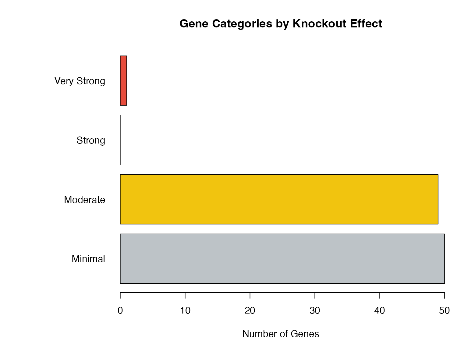


# Add text
cat("\nGene Categories:\n")
#> 
#> Gene Categories:
print(table(dr$category))
#> 
#>     Minimal    Moderate      Strong Very Strong 
#>          50          49           0           1

Potential Interpretations

Category	FC Range	Biological Meaning
Very Strong	>5	Direct targets, key pathway members
Strong	2-5	Secondary targets, co-regulated genes
Moderate	1-2	Indirectly affected genes
Minimal	<1	Background noise, unrelated genes

Quality Assessment

Check Knockout Gene Rank

ko_rank <- which(dr$gene == "G100")
cat("Knockout gene (G100) rank:", ko_rank, "\n")
#> Knockout gene (G100) rank: 1

if (ko_rank == 1) {
  cat("✓ PASS: Knockout gene is top-ranked (expected behavior)\n")
} else {
  cat("⚠ WARNING: Knockout gene is not top-ranked\n")
  cat("  This may indicate:\n")
  cat("  - Weak regulatory role of the knockout gene\n")
  cat("  - Need for parameter adjustment\n")
}
#> <U+2713> PASS: Knockout gene is top-ranked (expected behavior)

Network Sparsity Check

WT_sparsity <- 1 - sum(result$tensorNetworks$WT != 0) / prod(dim(result$tensorNetworks$WT))
cat("WT network sparsity:", round(WT_sparsity, 4), "\n")
#> WT network sparsity: 0.0657

if (WT_sparsity > 0.99) {
  cat("⚠ Network may be too sparse. Consider lowering q parameter.\n")
} else if (WT_sparsity < 0.8) {
  cat("⚠ Network may be too dense. Consider increasing q parameter.\n")
} else {
  cat("✓ Network sparsity is in acceptable range.\n")
}
#> <U+26A0> Network may be too dense. Consider increasing q parameter.

Significance Distribution

n_sig_005 <- sum(dr$p.adj < 0.05)
n_sig_001 <- sum(dr$p.adj < 0.01)
pct_sig <- round(n_sig_005 / nrow(dr) * 100, 1)

cat("Significant genes (FDR < 0.05):", n_sig_005, "(", pct_sig, "%)\n")
#> Significant genes (FDR < 0.05): 1 ( 1 %)
cat("Significant genes (FDR < 0.01):", n_sig_001, "\n")
#> Significant genes (FDR < 0.01): 1

if (pct_sig > 50) {
  cat("⚠ High proportion of significant genes. May indicate strong knockout effect or need for stricter thresholds.\n")
}

Exporting Results

# Export differential regulation table
write.csv(dr, "diffRegulation_results.csv", row.names = FALSE)

# Export significant genes only
sig_genes <- dr[dr$p.adj < 0.05, ]
write.csv(sig_genes, "significant_genes.csv", row.names = FALSE)

# Export networks as edge lists
WT_edges <- which(result$tensorNetworks$WT != 0, arr.ind = TRUE)
edge_list <- data.frame(
  from = rownames(result$tensorNetworks$WT)[WT_edges[, 1]],
  to = colnames(result$tensorNetworks$WT)[WT_edges[, 2]],
  weight = result$tensorNetworks$WT[WT_edges]
)
write.csv(edge_list, "WT_network_edges.csv", row.names = FALSE)

Summary

When interpreting scTenifoldKnk results:

Verify that the knockout gene ranks first
Examine the fold change distribution
Consider both statistical significance and effect size
Validate with known biology when possible
Use appropriate significance thresholds for your application

Session Info

sessionInfo()
#> R version 4.4.0 (2024-04-24)
#> Platform: aarch64-apple-darwin20
#> Running under: macOS 15.6.1
#> 
#> Matrix products: default
#> BLAS:   /Library/Frameworks/R.framework/Versions/4.4-arm64/Resources/lib/libRblas.0.dylib 
#> LAPACK: /Library/Frameworks/R.framework/Versions/4.4-arm64/Resources/lib/libRlapack.dylib;  LAPACK version 3.12.0
#> 
#> locale:
#> [1] C
#> 
#> time zone: Asia/Shanghai
#> tzcode source: internal
#> 
#> attached base packages:
#> [1] stats     graphics  grDevices utils     datasets  methods   base     
#> 
#> other attached packages:
#> [1] Matrix_1.7-4        scTenifoldKnk_2.1.0
#> 
#> loaded via a namespace (and not attached):
#>  [1] cli_3.6.5         knitr_1.51        rlang_1.1.7       xfun_0.56        
#>  [5] otel_0.2.0        textshaping_1.0.4 jsonlite_2.0.0    htmltools_0.5.9  
#>  [9] ragg_1.5.0        sass_0.4.10       rmarkdown_2.30    grid_4.4.0       
#> [13] evaluate_1.0.5    jquerylib_0.1.4   MASS_7.3-65       fastmap_1.2.0    
#> [17] yaml_2.3.12       lifecycle_1.0.5   compiler_4.4.0    RSpectra_0.16-2  
#> [21] fs_1.6.6          htmlwidgets_1.6.4 Rcpp_1.1.1        lattice_0.22-7   
#> [25] systemfonts_1.3.1 digest_0.6.39     R6_2.6.1          parallel_4.4.0   
#> [29] bslib_0.9.0       tools_4.4.0       pkgdown_2.1.3     cachem_1.1.0     
#> [33] desc_1.4.3

Zaoqu Liu

2026-01-23