Algorithm and Methodology

Zaoqu Liu

2026-01-24

Overview

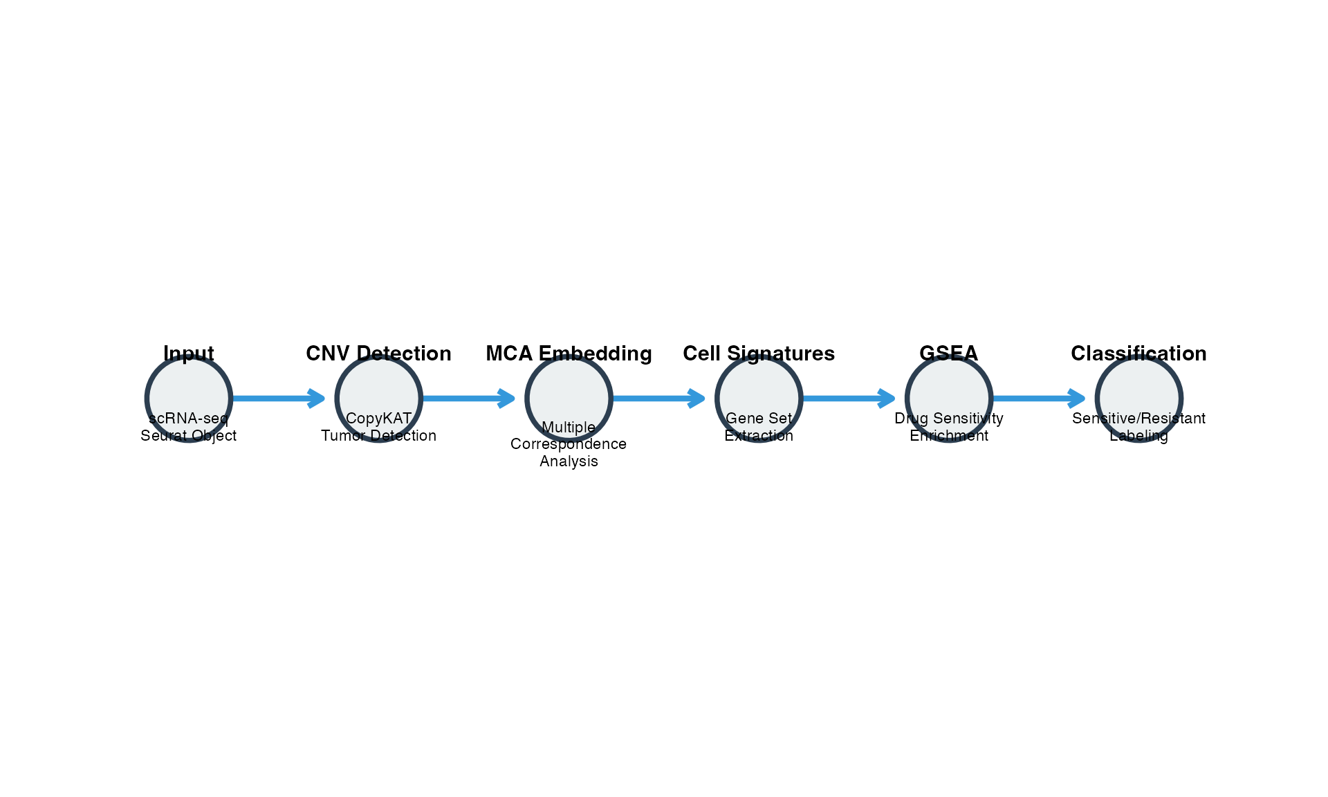
scPharm employs a multi-step computational pipeline to identify pharmacological subpopulations at single-cell resolution. This vignette describes the underlying algorithms and statistical methods.

Workflow Architecture

scPharm analytical workflow

Step 1: Copy Number Variation Detection

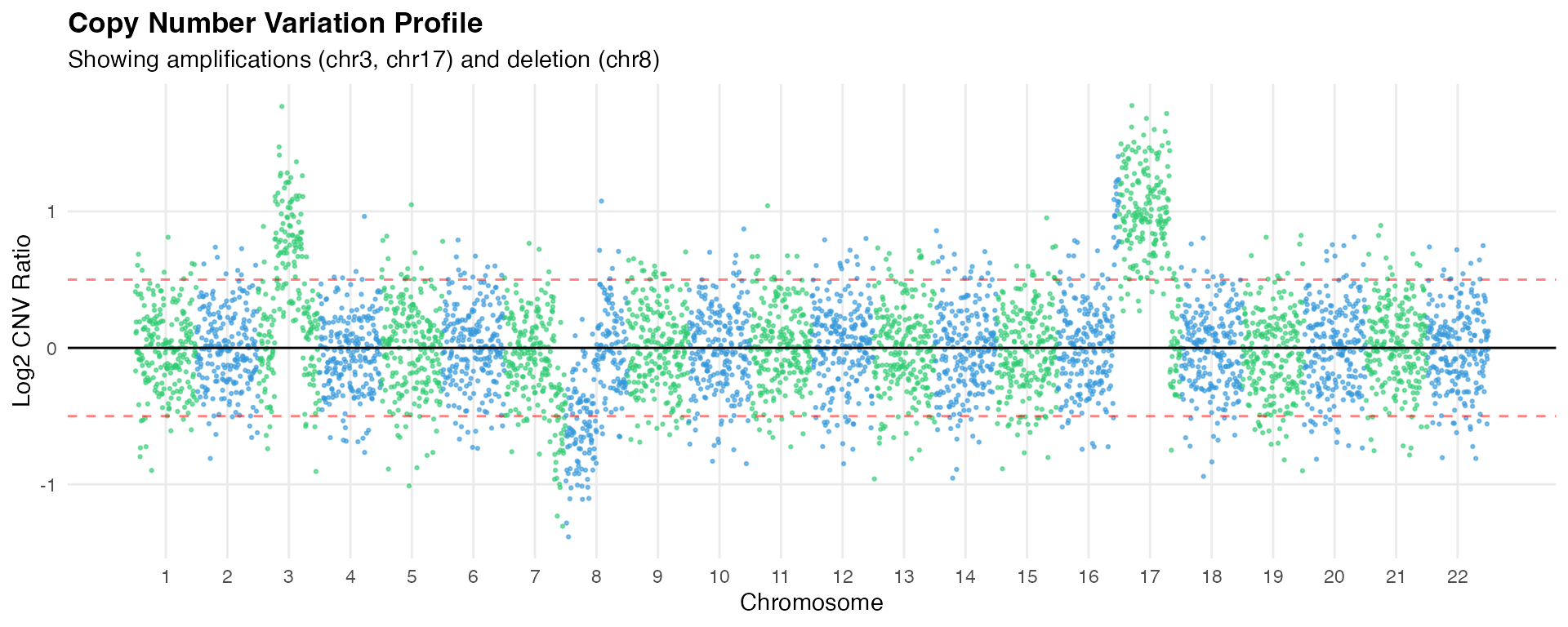
For tissue samples containing mixed tumor and normal cells, scPharm employs an integrated CopyKAT-based algorithm to distinguish malignant cells.

Algorithm Overview

The CNV detection follows these steps:

1. Gene Annotation: Map genes to chromosomal positions using hg20 annotations
2. Expression Binning: Aggregate expression into genomic bins (220 bins per chromosome)
3. Baseline Normalization: Use normal cells or synthetic baseline as reference
4. Smoothing: Apply Kalman filtering to reduce noise
5. Clustering: Hierarchical clustering to identify aneuploid populations

Mathematical Framework

For a gene $g$ at genomic position $p$, the relative copy number is estimated as:

$$\text{CNV}_{g} = \log_2\left(\frac{E_g^{tumor}}{E_g^{baseline}} + 1\right)$$

where $E_g$ represents the normalized expression level.

CNV profile across chromosomes

Step 2: Multiple Correspondence Analysis (MCA)

MCA is used for dimensionality reduction, preserving the correspondence between genes and cells.

Why MCA?

Unlike PCA which assumes continuous data, MCA is designed for categorical/count data and provides:

• Joint embedding of cells and genes
• Natural handling of sparse scRNA-seq data
• Interpretable gene-cell associations

Mathematical Formulation

Given a normalized expression matrix $\mathbf{X}$ with $n$ cells and $p$ genes:

1. Construct indicator matrix $\mathbf{Z}$ by discretizing expression levels
2. Compute correspondence matrix: $$\mathbf{S} = \mathbf{D}_r^{-1/2}(\mathbf{Z} - \mathbf{rc}^T)\mathbf{D}_c^{-1/2}$$
3. Perform SVD: $\mathbf{S} = \mathbf{U\Sigma V}^T$
4. Extract coordinates:
   • Cell coordinates: $\mathbf{F} = \mathbf{D}_r^{-1/2}\mathbf{U\Sigma}$
   • Gene coordinates: $\mathbf{G} = \mathbf{D}_c^{-1/2}\mathbf{V\Sigma}$

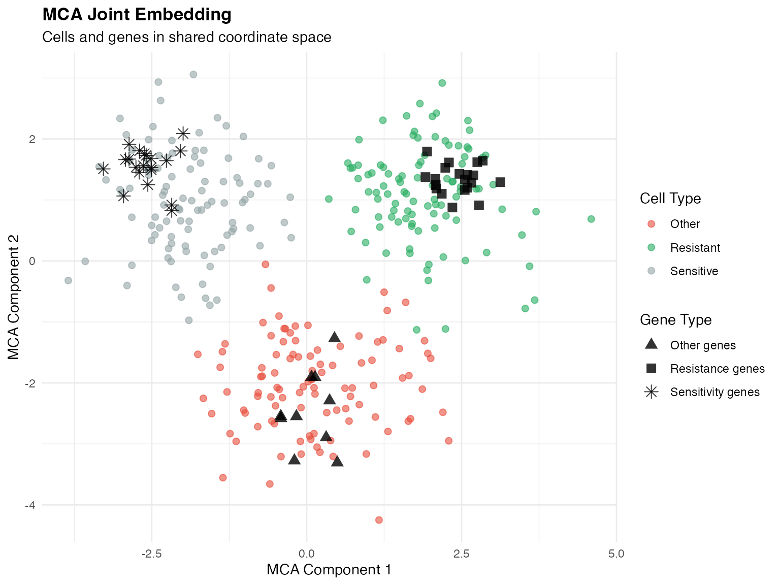
MCA embedding showing cell-gene correspondence

C++ Implementation

scPharm implements MCA using RcppArmadillo for computational efficiency:

// Simplified MCA computation (actual implementation in src/mca.cpp)
arma::mat SparseMCAStep1(arma::sp_mat& X) {
    // Column sums and total
    arma::vec col_sum = arma::vec(arma::sum(X, 0).t());
    double total = arma::accu(X);
    
    // Compute standardized residuals
    arma::mat Z = compute_residuals(X, col_sum, total);
    
    return Z;
}

Step 3: Cell Identity Signatures

For each cell, we extract a gene signature based on its position in MCA space.

Distance Metric

The association between cell $i$ and gene $j$ is computed as:

$$d_{ij} = \sqrt{\sum_{k=1}^{K} (F_{ik} - G_{jk})^2}$$

where $K$ is the number of MCA components.

Signature Extraction

For each cell, the top $n$ genes (by distance) form its identity signature:

$$\text{Signature}_i = \{g_1, g_2, ..., g_n\} \text{ where } d_{i,g_1} < d_{i,g_2} < ... < d_{i,g_n}$$

Step 4: Gene Set Enrichment Analysis

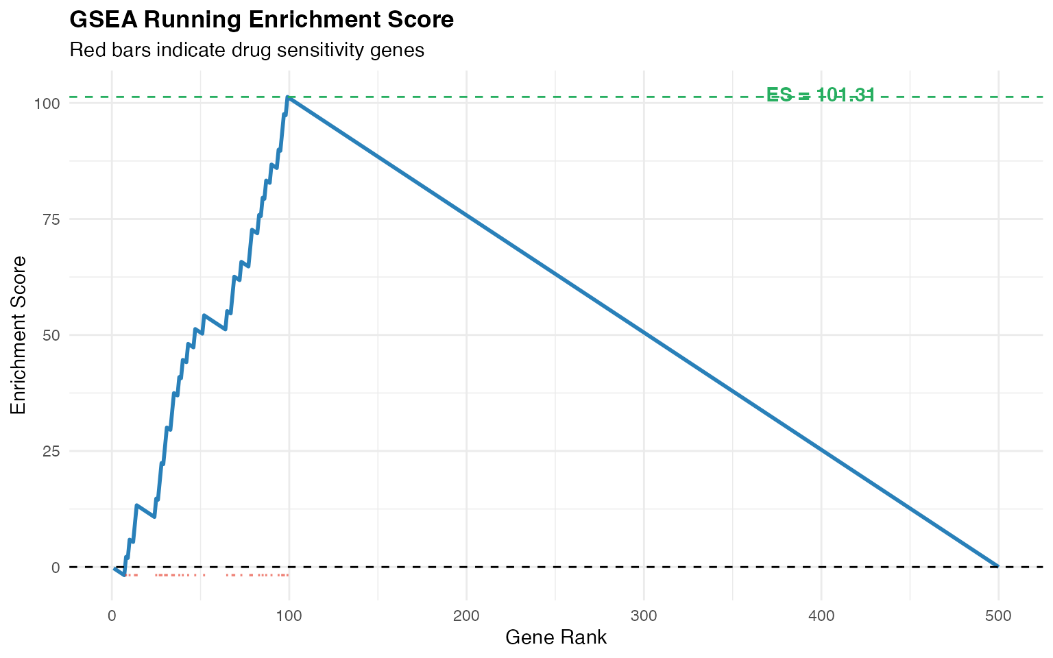
GSEA quantifies the enrichment of drug sensitivity genes within each cell’s signature.

GSEA Algorithm

1. Rank genes by their association with the cell
2. Calculate running enrichment score (ES): $$ES = \max_{j}\left(\sum_{g_i \in S, i \leq j} \sqrt{\frac{N-|S|}{|S|}} - \sum_{g_i \notin S, i \leq j} \sqrt{\frac{|S|}{N-|S|}}\right)$$
3. Normalize to obtain NES (Normalized Enrichment Score)

GSEA running enrichment score

Drug Sensitivity Gene Sets

Drug sensitivity gene sets are derived from GDSC2 database:

• For each drug, genes are ranked by correlation with IC50
• Top correlated genes → Sensitivity signature
• Bottom correlated genes → Resistance signature

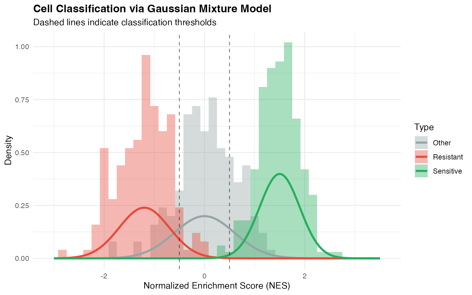
Step 5: Cell Classification

Gaussian Mixture Model

Cell NES values are modeled as a mixture of Gaussian distributions:

$$P(\text{NES}) = \pi_S \cdot \mathcal{N}(\mu_S, \sigma_S^2) + \pi_R \cdot \mathcal{N}(\mu_R, \sigma_R^2) + \pi_O \cdot \mathcal{N}(\mu_O, \sigma_O^2)$$

Gaussian Mixture Model for cell classification

Classification Criteria

Cells are classified based on NES thresholds:

Classification	Criterion
Sensitive	NES > threshold_s (default: 1.0)
Resistant	NES < threshold_r (default: -1.0)
Other	threshold_r ≤ NES ≤ threshold_s

Step 6: Drug Scoring Metrics

Drug Prioritization Score (Dr)

$$Dr = 1 - \left(\alpha \cdot \frac{n_S}{n_{tumor}} + \beta \cdot \overline{\text{NES}}_S\right)$$

where: - $n_S$ = number of sensitive cells - $n_{tumor}$ = total tumor cells - $\overline{\text{NES}}_S$ = mean NES of sensitive cells - $\alpha, \beta$ = weighting parameters

Interpretation: Lower Dr indicates better drug candidate.

Drug Side Effect Score (Dse)

$$Dse = \frac{n_{S,adj}}{n_{adj}} \cdot \overline{\text{NES}}_{S,adj}$$

where subscript $adj$ denotes adjacent (non-tumor) cells.

Interpretation: Higher Dse indicates more potential side effects.

Computational Complexity

Step	Complexity	Notes
CNV Detection	O(n × g)	n = cells, g = genes
MCA	O(min(n,g)³)	SVD computation
Cell Signatures	O(n × k)	k = MCA components
GSEA	O(n × d × g)	d = drugs
Classification	O(n × d)	GMM fitting

References

1. Gao R, et al. (2021). Delineating copy number and clonal substructure in human tumors from single-cell transcriptomes. Nature Biotechnology.

2. Subramanian A, et al. (2005). Gene set enrichment analysis: A knowledge-based approach. PNAS.

3. Yang W, et al. (2013). Genomics of Drug Sensitivity in Cancer (GDSC). Nucleic Acids Research.

4. Cortal A, et al. (2021). Gene signature extraction and cell identity recognition at the single-cell level with CelliD. Nature Biotechnology.

Session Info

sessionInfo()
#> R version 4.4.0 (2024-04-24)
#> Platform: aarch64-apple-darwin20
#> Running under: macOS 15.6.1
#> 
#> Matrix products: default
#> BLAS:   /Library/Frameworks/R.framework/Versions/4.4-arm64/Resources/lib/libRblas.0.dylib 
#> LAPACK: /Library/Frameworks/R.framework/Versions/4.4-arm64/Resources/lib/libRlapack.dylib;  LAPACK version 3.12.0
#> 
#> locale:
#> [1] C
#> 
#> time zone: Asia/Shanghai
#> tzcode source: internal
#> 
#> attached base packages:
#> [1] stats     graphics  grDevices utils     datasets  methods   base     
#> 
#> other attached packages:
#> [1] dplyr_1.1.4   ggplot2_4.0.1
#> 
#> loaded via a namespace (and not attached):
#>  [1] gtable_0.3.6       jsonlite_2.0.0     compiler_4.4.0     tidyselect_1.2.1  
#>  [5] dichromat_2.0-0.1  jquerylib_0.1.4    systemfonts_1.3.1  scales_1.4.0      
#>  [9] textshaping_1.0.4  yaml_2.3.12        fastmap_1.2.0      R6_2.6.1          
#> [13] labeling_0.4.3     generics_0.1.4     knitr_1.51         htmlwidgets_1.6.4 
#> [17] tibble_3.3.1       desc_1.4.3         bslib_0.9.0        pillar_1.11.1     
#> [21] RColorBrewer_1.1-3 rlang_1.1.7        cachem_1.1.0       xfun_0.56         
#> [25] fs_1.6.6           sass_0.4.10        S7_0.2.1           otel_0.2.0        
#> [29] cli_3.6.5          pkgdown_2.1.3      withr_3.0.2        magrittr_2.0.4    
#> [33] digest_0.6.39      grid_4.4.0         lifecycle_1.0.5    vctrs_0.7.1       
#> [37] evaluate_1.0.5     glue_1.8.0         farver_2.1.2       ragg_1.5.0        
#> [41] rmarkdown_2.30     tools_4.4.0        pkgconfig_2.0.3    htmltools_0.5.9