Introduction
This vignette demonstrates various visualization strategies for scPharm analysis results. Effective visualization is crucial for interpreting pharmacological heterogeneity at single-cell resolution.
Simulated Analysis Results
For demonstration, we create simulated scPharm results.
set.seed(42)
n_cells <- 500

# Simulate UMAP coordinates
umap_data <- data.frame(
  UMAP1 = c(rnorm(200, -3, 1), rnorm(150, 3, 1), rnorm(150, 0, 1.5)),
  UMAP2 = c(rnorm(200, 2, 1), rnorm(150, 2, 1), rnorm(150, -2, 1.2)),
  cell_label = c(rep("tumor", 350), rep("adjacent", 150)),
  drug_label = c(
    rep("sensitive", 150), rep("resistant", 100), rep("other", 100),
    sample(c("sensitive", "resistant", "other"), 150,
           replace = TRUE, prob = c(0.1, 0.1, 0.8))
  ),
  NES = c(
    rnorm(150, 1.5, 0.4),   # Sensitive tumor
    rnorm(100, -1.2, 0.4),  # Resistant tumor
    rnorm(100, 0, 0.5),     # Other tumor
    rnorm(150, 0, 0.6)      # Adjacent
  ),
  cell_id = paste0("Cell_", 1:n_cells)
)

# Drug ranking data
drug_ranking <- data.frame(
  DRUG_NAME = c("Docetaxel", "Paclitaxel", "Erlotinib", "Gefitinib",
                "Tamoxifen", "Cisplatin", "Doxorubicin", "Imatinib"),
  Dr = c(0.15, 0.22, 0.35, 0.42, 0.55, 0.61, 0.72, 0.85),
  Dse = c(0.25, 0.18, 0.45, 0.32, 0.12, 0.55, 0.48, 0.22),
  sensitive_pct = c(0.42, 0.38, 0.32, 0.28, 0.22, 0.20, 0.15, 0.08)
)
1. Cell Type Distribution
UMAP with Cell Labels
ggplot(umap_data, aes(x = UMAP1, y = UMAP2, color = cell_label)) +
  geom_point(size = 1.5, alpha = 0.7) +
  scale_color_manual(
    values = c("tumor" = scpharm_colors$tumor,
               "adjacent" = scpharm_colors$adjacent),
    name = "Cell Type"
  ) +
  labs(
    title = "Cell Type Distribution",
    subtitle = "Tumor vs Adjacent cells identified by CNV analysis",
    x = "UMAP 1", y = "UMAP 2"
  ) +
  theme_minimal() +
  theme(
    plot.title = element_text(face = "bold", size = 14),
    legend.position = "right"
  ) +
  guides(color = guide_legend(override.aes = list(size = 4)))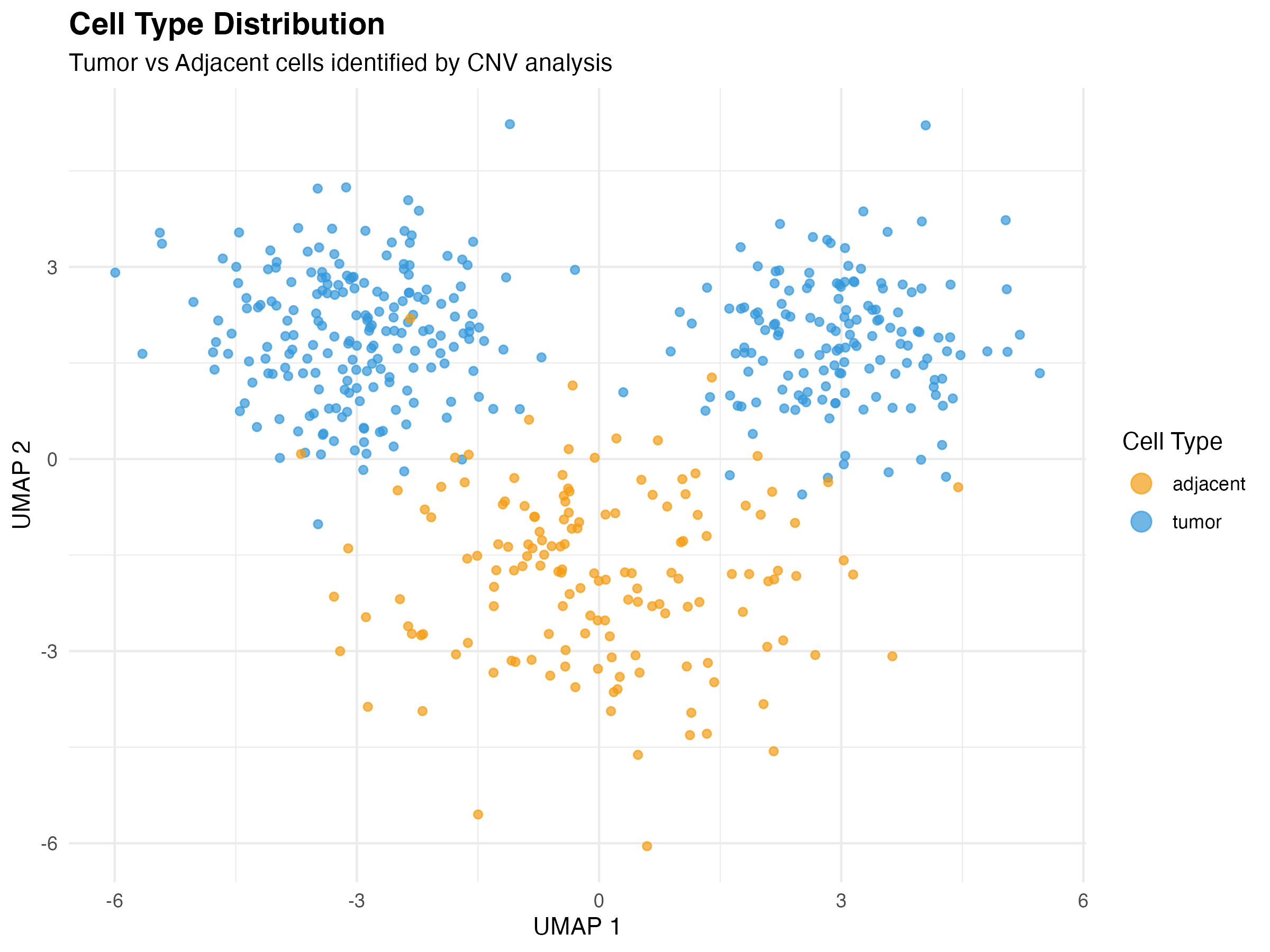
UMAP visualization colored by cell type
UMAP with Drug Response
ggplot(umap_data, aes(x = UMAP1, y = UMAP2, color = drug_label)) +
  geom_point(size = 1.5, alpha = 0.7) +
  scale_color_manual(
    values = c("sensitive" = scpharm_colors$sensitive,
               "resistant" = scpharm_colors$resistant,
               "other" = scpharm_colors$other),
    name = "Drug Response"
  ) +
  labs(
    title = "Pharmacological Subpopulations",
    subtitle = "Drug sensitivity classification for Docetaxel",
    x = "UMAP 1", y = "UMAP 2"
  ) +
  theme_minimal() +
  theme(
    plot.title = element_text(face = "bold", size = 14),
    legend.position = "right"
  ) +
  guides(color = guide_legend(override.aes = list(size = 4)))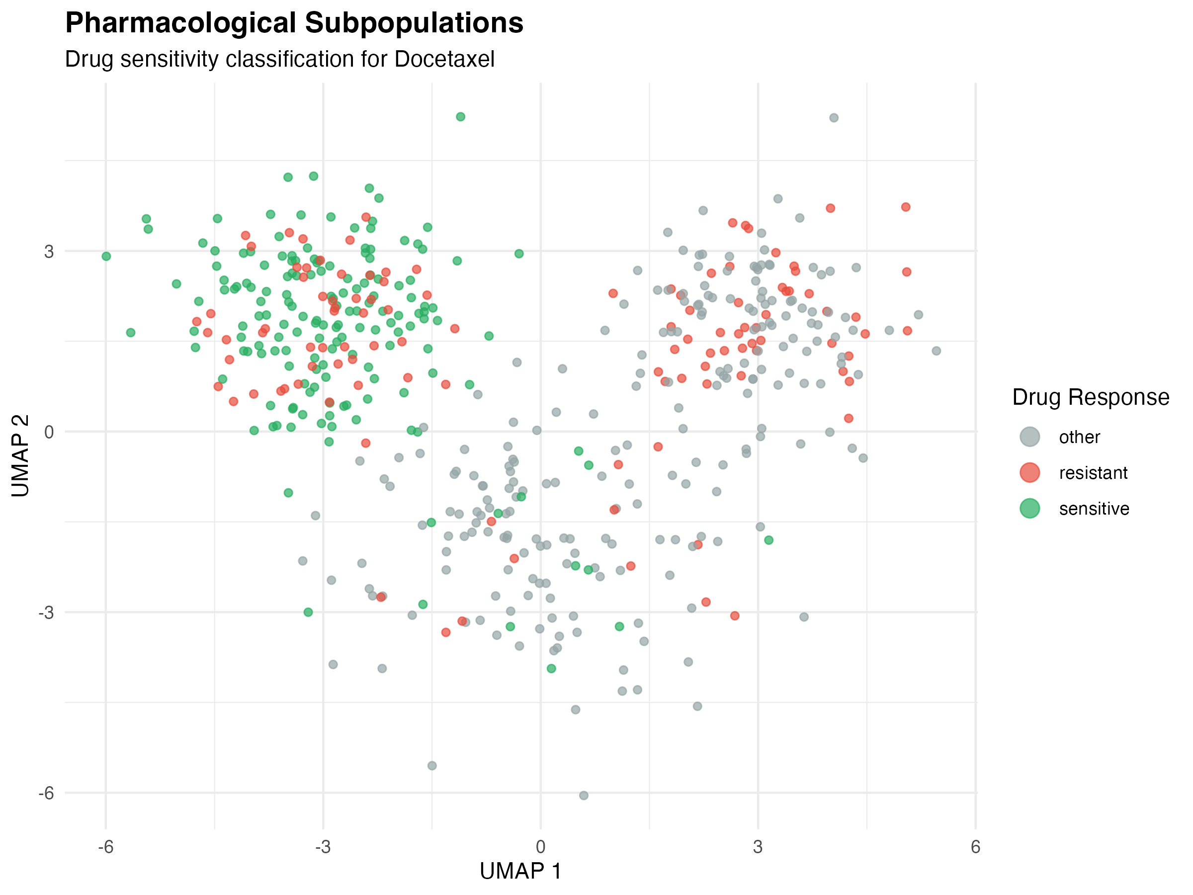
UMAP visualization colored by drug response
UMAP with NES Values
ggplot(umap_data, aes(x = UMAP1, y = UMAP2, color = NES)) +
  geom_point(size = 1.5, alpha = 0.8) +
  scale_color_gradient2(
    low = scpharm_colors$resistant,
    mid = "white",
    high = scpharm_colors$sensitive,
    midpoint = 0,
    name = "NES"
  ) +
  labs(
    title = "Drug Sensitivity Enrichment",
    subtitle = "Normalized Enrichment Score (NES) distribution",
    x = "UMAP 1", y = "UMAP 2"
  ) +
  theme_minimal() +
  theme(
    plot.title = element_text(face = "bold", size = 14),
    legend.position = "right"
  )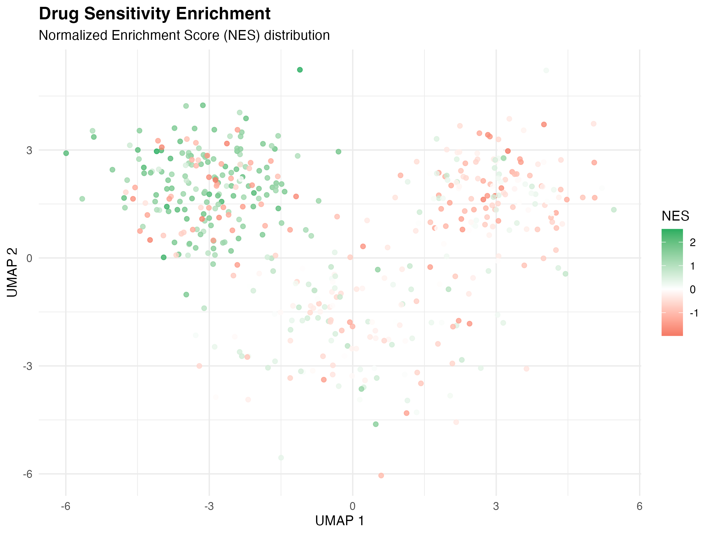
UMAP visualization colored by NES
2. NES Distribution Analysis
Histogram by Cell Type
ggplot(umap_data, aes(x = NES, fill = cell_label)) +
  geom_histogram(bins = 40, alpha = 0.7, position = "identity") +
  geom_vline(xintercept = c(-1, 1), linetype = "dashed", alpha = 0.5) +
  scale_fill_manual(
    values = c("tumor" = scpharm_colors$tumor,
               "adjacent" = scpharm_colors$adjacent),
    name = "Cell Type"
  ) +
  annotate("text", x = -1.5, y = 40, label = "Resistant\nThreshold",
           size = 3, color = "gray40") +
  annotate("text", x = 1.5, y = 40, label = "Sensitive\nThreshold",
           size = 3, color = "gray40") +
  labs(
    title = "NES Distribution by Cell Type",
    x = "Normalized Enrichment Score (NES)",
    y = "Count"
  ) +
  theme_minimal() +
  theme(plot.title = element_text(face = "bold", size = 14))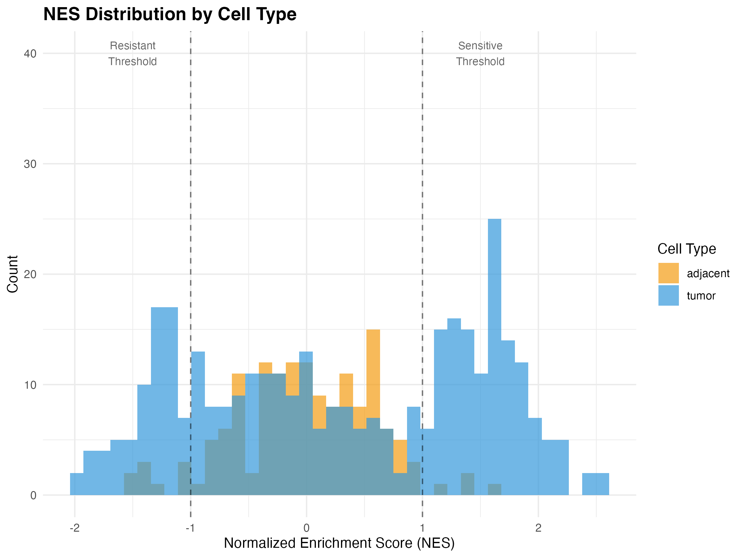
NES distribution histogram
Density Plot
tumor_data <- umap_data[umap_data$cell_label == "tumor", ]

ggplot(tumor_data, aes(x = NES, fill = drug_label, color = drug_label)) +
  geom_density(alpha = 0.4, size = 1) +
  scale_fill_manual(
    values = c("sensitive" = scpharm_colors$sensitive,
               "resistant" = scpharm_colors$resistant,
               "other" = scpharm_colors$other),
    name = "Classification"
  ) +
  scale_color_manual(
    values = c("sensitive" = scpharm_colors$sensitive,
               "resistant" = scpharm_colors$resistant,
               "other" = scpharm_colors$other),
    name = "Classification"
  ) +
  labs(
    title = "NES Density Distribution (Tumor Cells)",
    x = "Normalized Enrichment Score (NES)",
    y = "Density"
  ) +
  theme_minimal() +
  theme(plot.title = element_text(face = "bold", size = 14))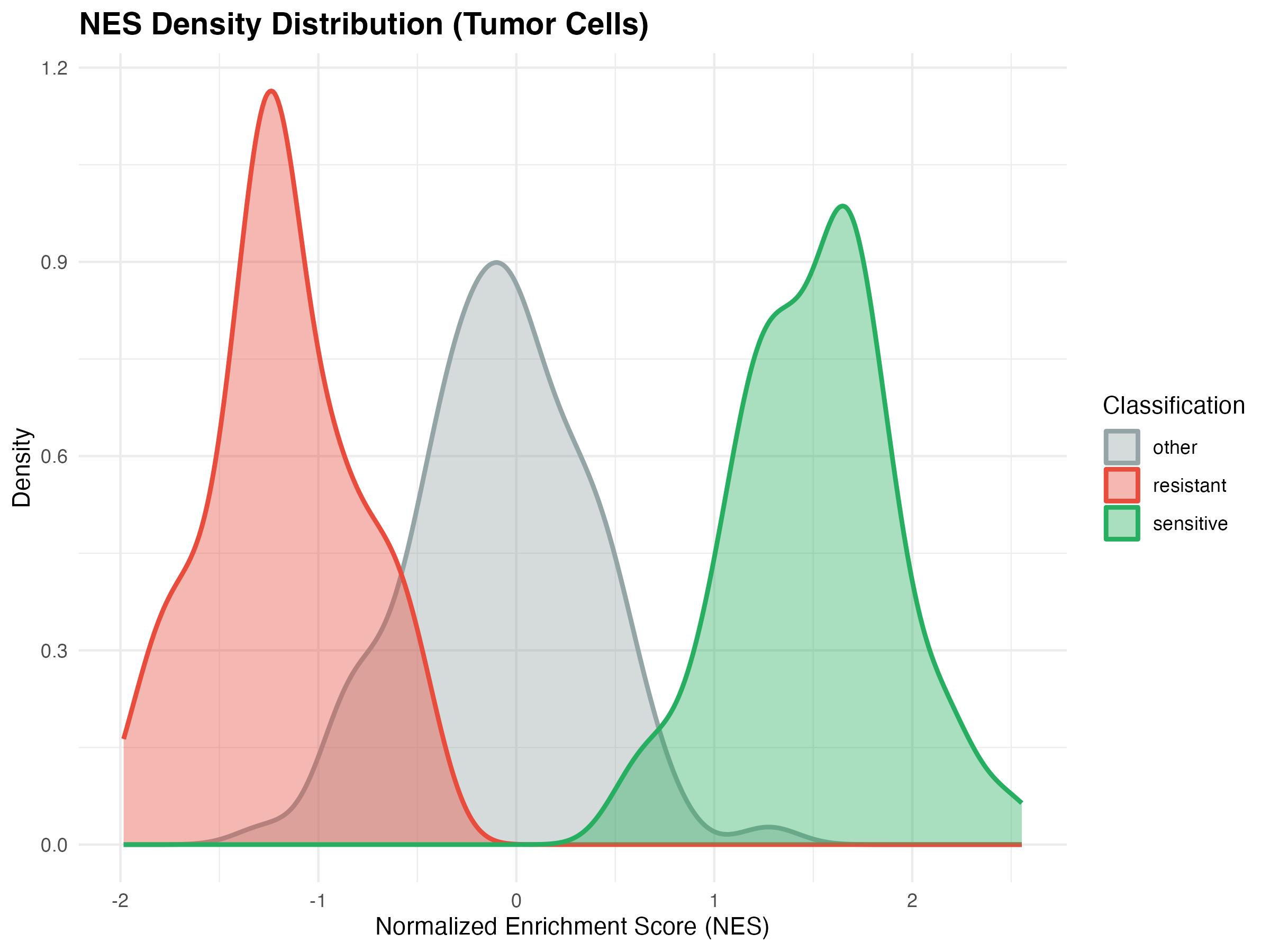
NES density by drug response classification
Violin Plot
ggplot(umap_data, aes(x = interaction(cell_label, drug_label),
                       y = NES, fill = drug_label)) +
  geom_violin(alpha = 0.7, scale = "width") +
  geom_boxplot(width = 0.2, outlier.size = 0.5, alpha = 0.8) +
  scale_fill_manual(
    values = c("sensitive" = scpharm_colors$sensitive,
               "resistant" = scpharm_colors$resistant,
               "other" = scpharm_colors$other),
    name = "Drug Response"
  ) +
  labs(
    title = "NES Distribution by Cell Type and Drug Response",
    x = "Cell Type × Drug Response",
    y = "NES"
  ) +
  theme_minimal() +
  theme(
    plot.title = element_text(face = "bold", size = 14),
    axis.text.x = element_text(angle = 45, hjust = 1)
  )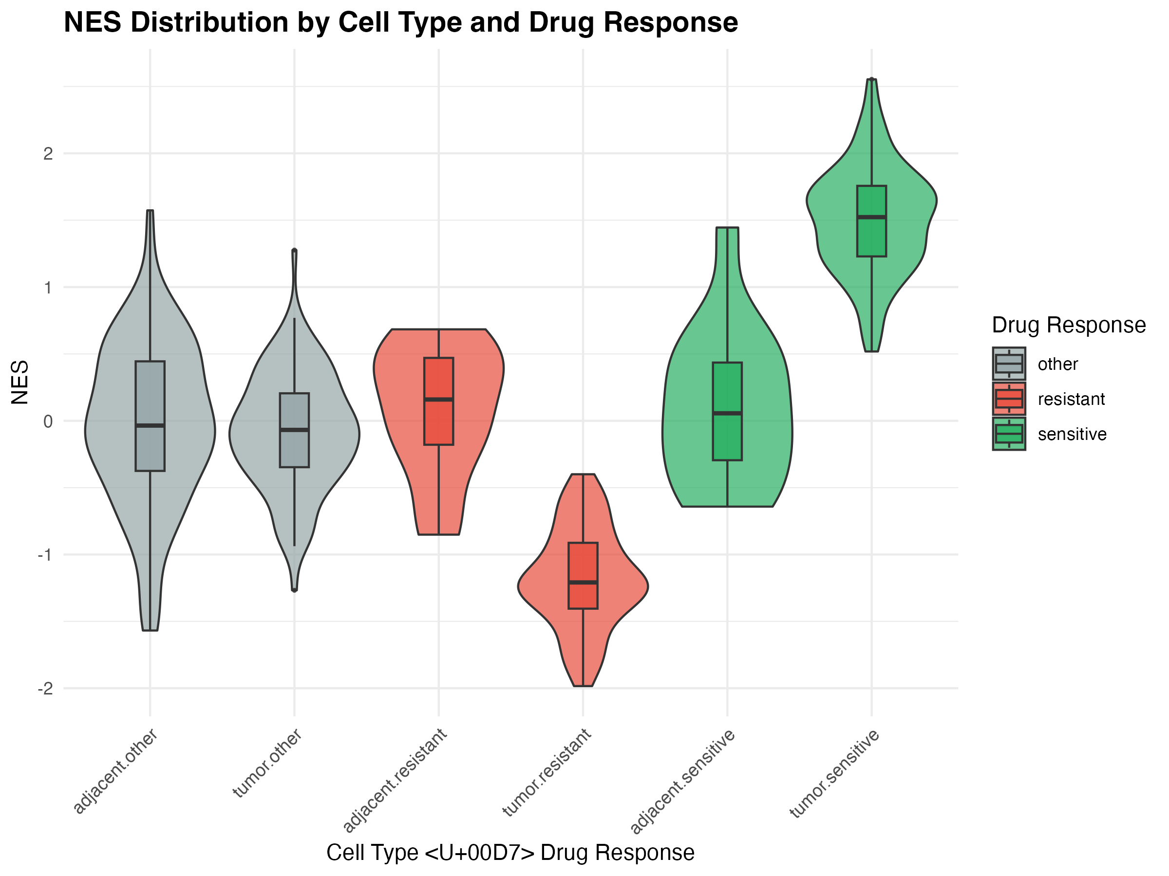
NES violin plot by cell type and drug response
3. Drug Prioritization Visualization
Bar Plot of Dr Scores
drug_ranking <- drug_ranking[order(drug_ranking$Dr), ]
drug_ranking$DRUG_NAME <- factor(drug_ranking$DRUG_NAME,
                                  levels = drug_ranking$DRUG_NAME)

ggplot(drug_ranking, aes(x = DRUG_NAME, y = Dr, fill = Dr)) +
  geom_col(width = 0.7) +
  geom_text(aes(label = sprintf("%.2f", Dr)),
            vjust = -0.5, size = 3.5) +
  scale_fill_gradient(low = scpharm_colors$sensitive,
                      high = scpharm_colors$resistant,
                      name = "Dr Score") +
  labs(
    title = "Drug Prioritization Ranking",
    subtitle = "Lower Dr score indicates better drug candidate",
    x = "Drug",
    y = "Drug Prioritization Score (Dr)"
  ) +
  theme_minimal() +
  theme(
    plot.title = element_text(face = "bold", size = 14),
    axis.text.x = element_text(angle = 45, hjust = 1)
  ) +
  coord_cartesian(ylim = c(0, 1))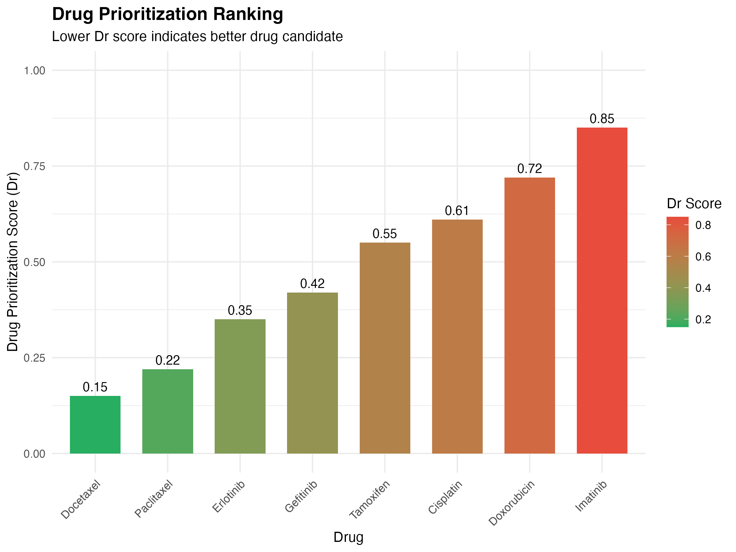
Drug prioritization ranking
Dr vs Dse Scatter Plot
ggplot(drug_ranking, aes(x = Dr, y = Dse, label = DRUG_NAME)) +
  geom_point(aes(size = sensitive_pct, color = Dr), alpha = 0.8) +
  geom_text(vjust = -1.2, size = 3.5) +
  geom_hline(yintercept = 0.3, linetype = "dashed", alpha = 0.5) +
  geom_vline(xintercept = 0.4, linetype = "dashed", alpha = 0.5) +
  scale_color_gradient(low = scpharm_colors$sensitive,
                       high = scpharm_colors$resistant,
                       name = "Dr Score") +
  scale_size_continuous(range = c(3, 12), name = "Sensitive %") +
  annotate("rect", xmin = 0, xmax = 0.4, ymin = 0, ymax = 0.3,
           fill = scpharm_colors$sensitive, alpha = 0.1) +
  annotate("text", x = 0.2, y = 0.15, label = "Optimal\nRegion",
           size = 4, fontface = "bold", color = scpharm_colors$sensitive) +
  labs(
    title = "Drug Efficacy vs Side Effects",
    subtitle = "Optimal drugs: low Dr (effective) and low Dse (safe)",
    x = "Drug Prioritization Score (Dr)",
    y = "Drug Side Effect Score (Dse)"
  ) +
  theme_minimal() +
  theme(
    plot.title = element_text(face = "bold", size = 14),
    legend.position = "right"
  ) +
  coord_cartesian(xlim = c(0, 1), ylim = c(0, 0.7))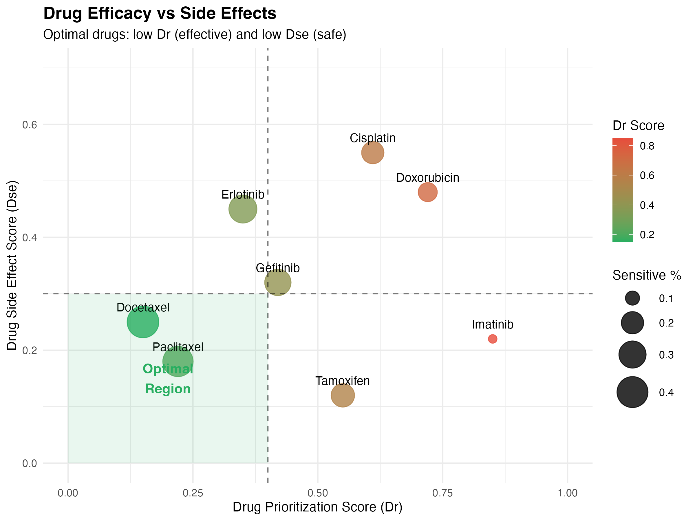
Drug efficacy vs side effects
4. Cell Proportion Analysis
Stacked Bar Plot
# Calculate proportions
prop_data <- umap_data %>%
  filter(cell_label == "tumor") %>%
  count(drug_label) %>%
  mutate(pct = n / sum(n) * 100)

ggplot(prop_data, aes(x = "", y = pct, fill = drug_label)) +
  geom_col(width = 0.6) +
  geom_text(aes(label = sprintf("%.1f%%", pct)),
            position = position_stack(vjust = 0.5),
            color = "white", fontface = "bold", size = 5) +
  scale_fill_manual(
    values = c("sensitive" = scpharm_colors$sensitive,
               "resistant" = scpharm_colors$resistant,
               "other" = scpharm_colors$other),
    name = "Drug Response"
  ) +
  labs(
    title = "Tumor Cell Composition",
    subtitle = "Proportion of cells by drug response classification",
    y = "Percentage (%)"
  ) +
  theme_minimal() +
  theme(
    plot.title = element_text(face = "bold", size = 14),
    axis.title.x = element_blank(),
    axis.text.x = element_blank()
  ) +
  coord_flip()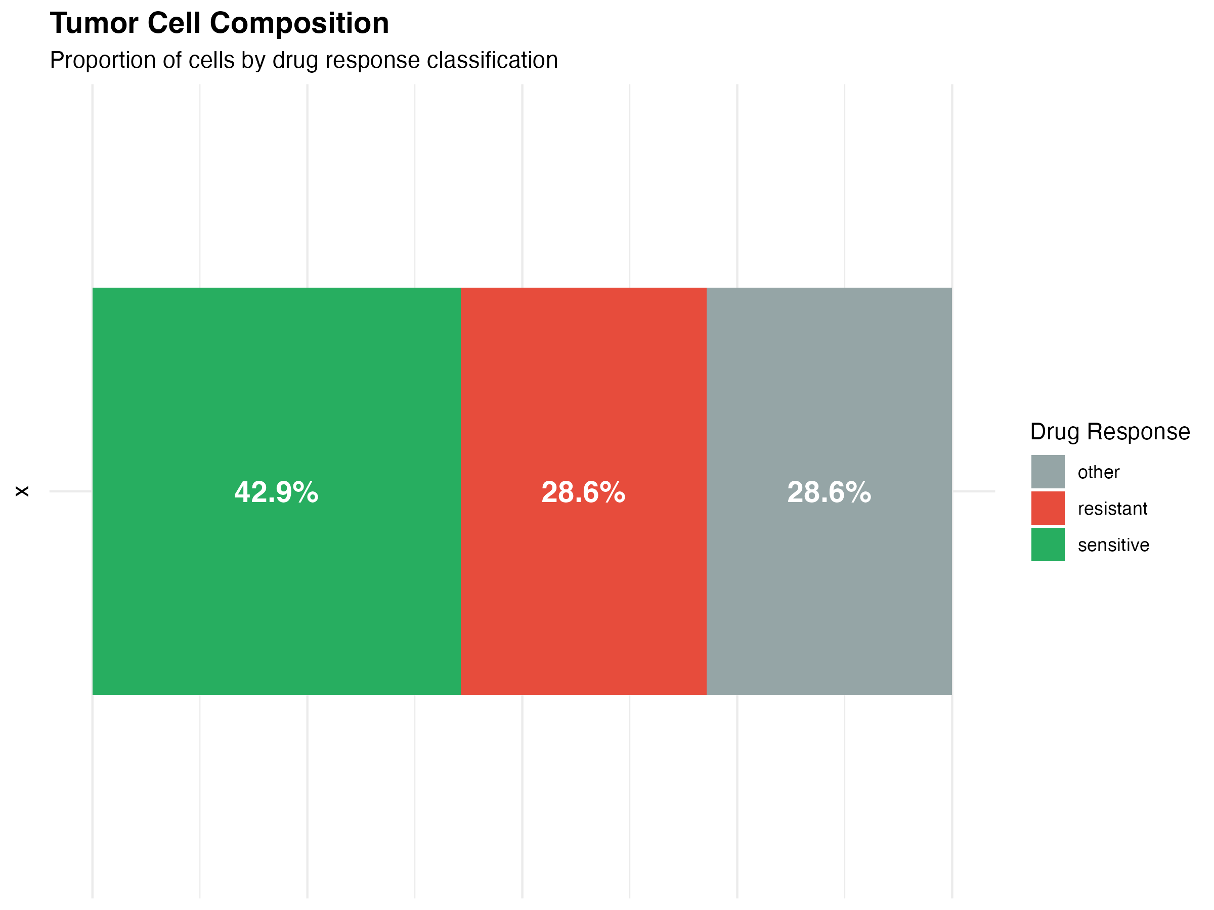
Cell proportion by drug response
Pie Chart
ggplot(prop_data, aes(x = "", y = pct, fill = drug_label)) +
  geom_col(width = 1) +
  coord_polar(theta = "y") +
  geom_text(aes(label = sprintf("%s\n%.1f%%", drug_label, pct)),
            position = position_stack(vjust = 0.5),
            color = "white", fontface = "bold", size = 4) +
  scale_fill_manual(
    values = c("sensitive" = scpharm_colors$sensitive,
               "resistant" = scpharm_colors$resistant,
               "other" = scpharm_colors$other)
  ) +
  labs(title = "Drug Response Distribution") +
  theme_void() +
  theme(
    plot.title = element_text(face = "bold", size = 14, hjust = 0.5),
    legend.position = "none"
  )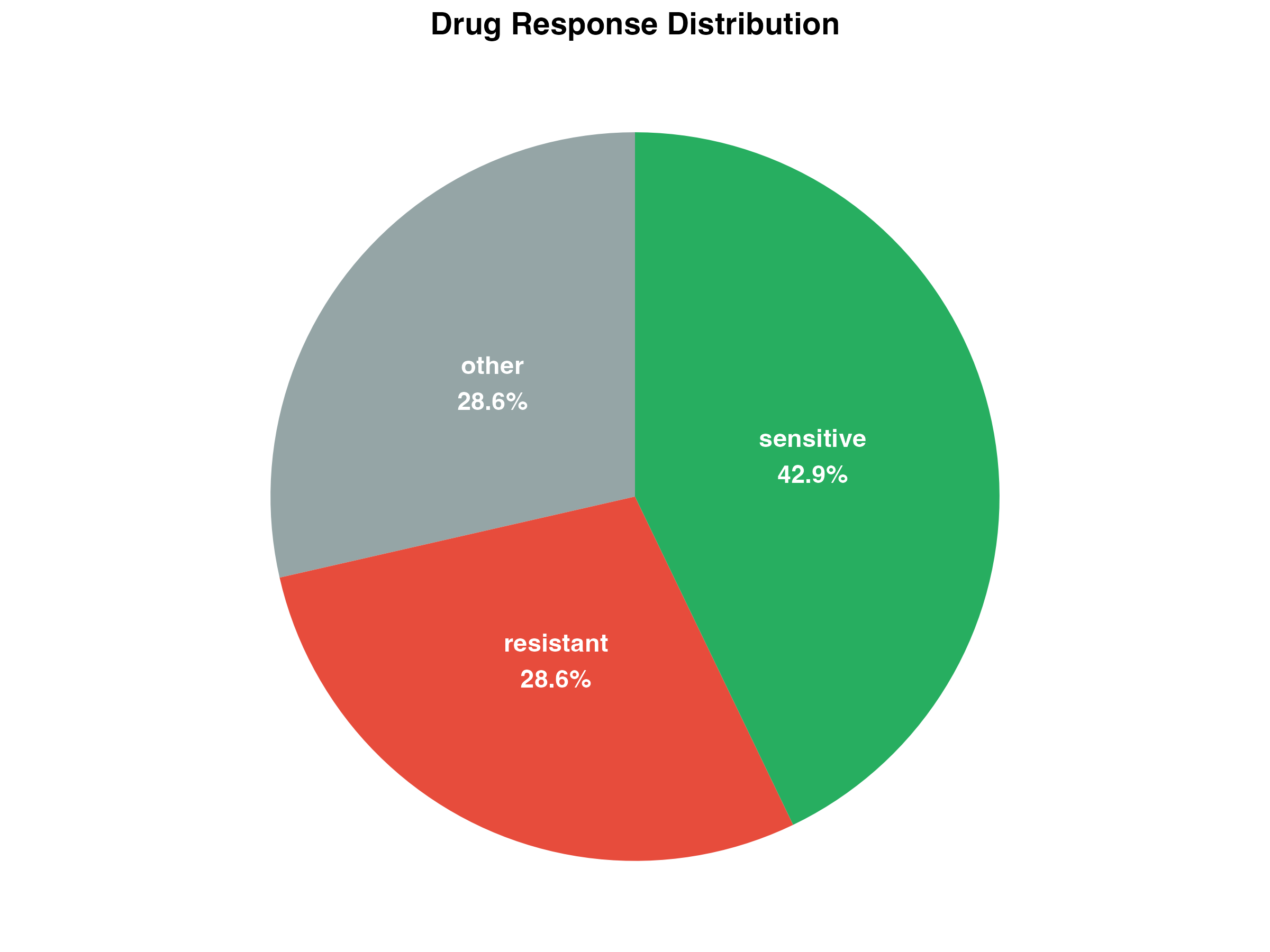
Pie chart of cell proportions
5. Multi-Drug Comparison
Heatmap of Drug Effects
# Simulate multi-drug data
set.seed(123)
drugs <- c("Docetaxel", "Paclitaxel", "Erlotinib", "Tamoxifen", "Cisplatin")
clusters <- paste0("Cluster_", 1:8)

heatmap_data <- expand.grid(Drug = drugs, Cluster = clusters) %>%
  mutate(
    Mean_NES = rnorm(n(), 0, 0.8),
    Mean_NES = case_when(
      Drug == "Docetaxel" & Cluster %in% c("Cluster_1", "Cluster_2") ~ Mean_NES + 1.5,
      Drug == "Paclitaxel" & Cluster %in% c("Cluster_1", "Cluster_3") ~ Mean_NES + 1.2,
      Drug == "Erlotinib" & Cluster %in% c("Cluster_4", "Cluster_5") ~ Mean_NES + 1.0,
      Drug == "Cisplatin" & Cluster %in% c("Cluster_6", "Cluster_7") ~ Mean_NES - 1.0,
      TRUE ~ Mean_NES
    )
  )

ggplot(heatmap_data, aes(x = Cluster, y = Drug, fill = Mean_NES)) +
  geom_tile(color = "white", size = 0.5) +
  geom_text(aes(label = sprintf("%.1f", Mean_NES)),
            size = 3, color = "black") +
  scale_fill_gradient2(
    low = scpharm_colors$resistant,
    mid = "white",
    high = scpharm_colors$sensitive,
    midpoint = 0,
    name = "Mean NES"
  ) +
  labs(
    title = "Drug Sensitivity Across Cell Clusters",
    subtitle = "Mean NES values per drug-cluster combination",
    x = "Cell Cluster",
    y = "Drug"
  ) +
  theme_minimal() +
  theme(
    plot.title = element_text(face = "bold", size = 14),
    axis.text.x = element_text(angle = 45, hjust = 1),
    panel.grid = element_blank()
  )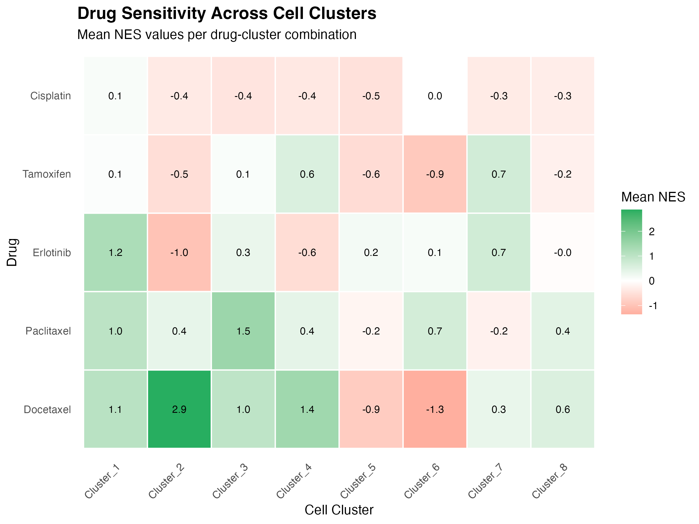
Heatmap of drug effects across cell clusters
6. Combined Dashboard
Summary Panel
# Panel A: UMAP with drug response
p1 <- ggplot(umap_data, aes(x = UMAP1, y = UMAP2, color = drug_label)) +
  geom_point(size = 1, alpha = 0.7) +
  scale_color_manual(
    values = c("sensitive" = scpharm_colors$sensitive,
               "resistant" = scpharm_colors$resistant,
               "other" = scpharm_colors$other),
    name = "Response"
  ) +
  labs(title = "A. Drug Response UMAP", x = "UMAP 1", y = "UMAP 2") +
  theme_minimal() +
  theme(plot.title = element_text(face = "bold", size = 12),
        legend.position = "bottom")

# Panel B: NES distribution
p2 <- ggplot(tumor_data, aes(x = NES, fill = drug_label)) +
  geom_histogram(bins = 30, alpha = 0.7, position = "identity") +
  scale_fill_manual(
    values = c("sensitive" = scpharm_colors$sensitive,
               "resistant" = scpharm_colors$resistant,
               "other" = scpharm_colors$other),
    name = "Response"
  ) +
  labs(title = "B. NES Distribution", x = "NES", y = "Count") +
  theme_minimal() +
  theme(plot.title = element_text(face = "bold", size = 12),
        legend.position = "bottom")

# Panel C: Drug ranking
p3 <- ggplot(drug_ranking, aes(x = DRUG_NAME, y = Dr, fill = Dr)) +
  geom_col(width = 0.7) +
  scale_fill_gradient(low = scpharm_colors$sensitive,
                      high = scpharm_colors$resistant,
                      guide = "none") +
  labs(title = "C. Drug Ranking", x = "Drug", y = "Dr Score") +
  theme_minimal() +
  theme(plot.title = element_text(face = "bold", size = 12),
        axis.text.x = element_text(angle = 45, hjust = 1))

# Panel D: Cell proportions
p4 <- ggplot(prop_data, aes(x = "", y = pct, fill = drug_label)) +
  geom_col(width = 1) +
  coord_polar(theta = "y") +
  scale_fill_manual(
    values = c("sensitive" = scpharm_colors$sensitive,
               "resistant" = scpharm_colors$resistant,
               "other" = scpharm_colors$other),
    name = "Response"
  ) +
  labs(title = "D. Cell Proportions") +
  theme_void() +
  theme(plot.title = element_text(face = "bold", size = 12, hjust = 0.5),
        legend.position = "bottom")

# Combine panels
(p1 | p2) / (p3 | p4) +
  plot_annotation(
    title = "scPharm Analysis Summary",
    subtitle = "Comprehensive visualization of pharmacological heterogeneity",
    theme = theme(
      plot.title = element_text(face = "bold", size = 16),
      plot.subtitle = element_text(size = 12, color = "gray40")
    )
  )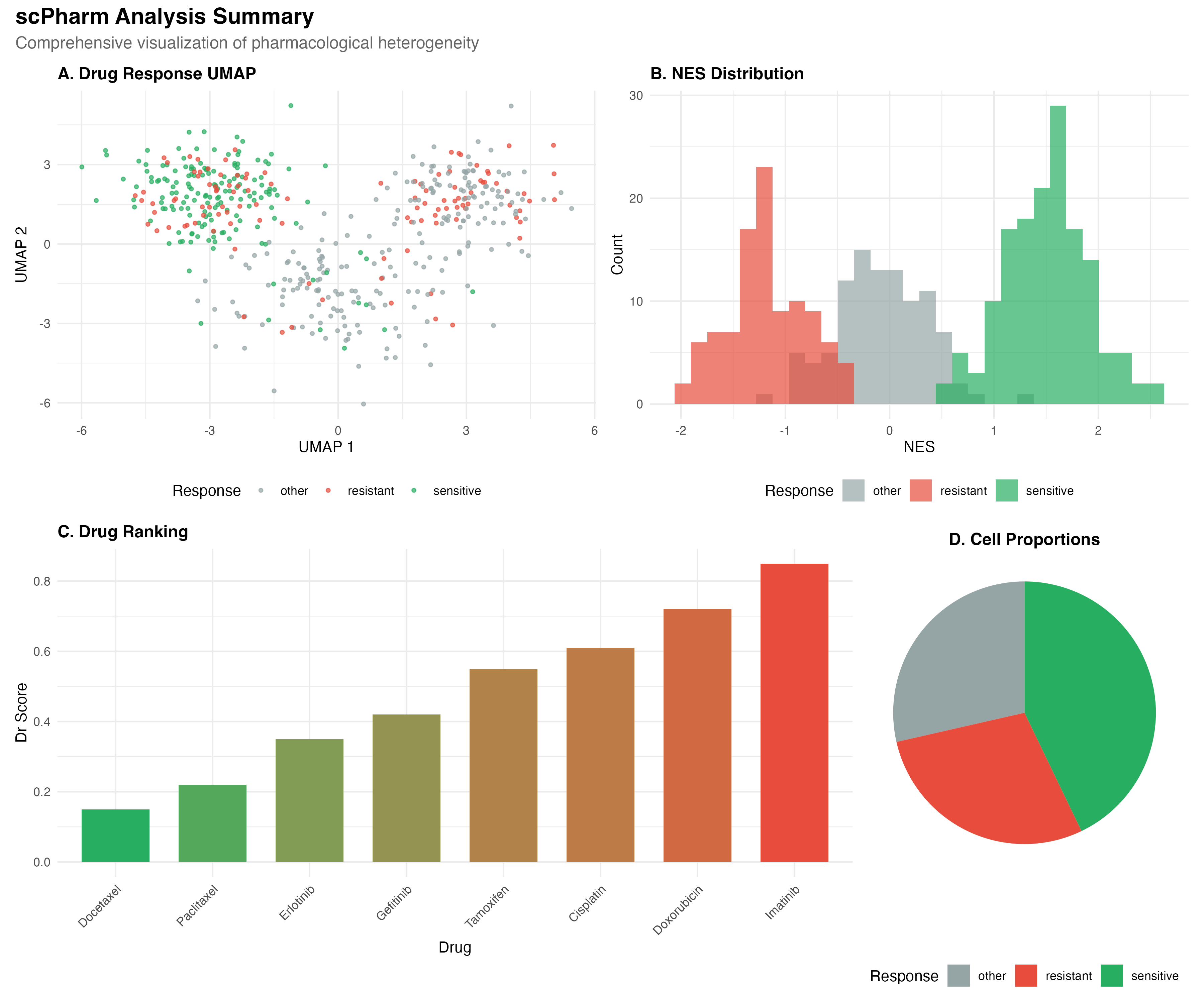
Combined analysis dashboard
Session Info
sessionInfo()
#> R version 4.4.0 (2024-04-24)
#> Platform: aarch64-apple-darwin20
#> Running under: macOS 15.6.1
#>
#> Matrix products: default
#> BLAS:   /Library/Frameworks/R.framework/Versions/4.4-arm64/Resources/lib/libRblas.0.dylib
#> LAPACK: /Library/Frameworks/R.framework/Versions/4.4-arm64/Resources/lib/libRlapack.dylib;  LAPACK version 3.12.0
#>
#> locale:
#> [1] C
#>
#> time zone: Asia/Shanghai
#> tzcode source: internal
#>
#> attached base packages:
#> [1] stats     graphics  grDevices utils     datasets  methods   base
#>
#> other attached packages:
#> [1] patchwork_1.3.2 tidyr_1.3.2     dplyr_1.1.4     ggplot2_4.0.1
#>
#> loaded via a namespace (and not attached):
#>  [1] gtable_0.3.6       jsonlite_2.0.0     compiler_4.4.0     tidyselect_1.2.1
#>  [5] dichromat_2.0-0.1  jquerylib_0.1.4    systemfonts_1.3.1  scales_1.4.0
#>  [9] textshaping_1.0.4  yaml_2.3.12        fastmap_1.2.0      R6_2.6.1
#> [13] labeling_0.4.3     generics_0.1.4     knitr_1.51         htmlwidgets_1.6.4
#> [17] tibble_3.3.1       desc_1.4.3         bslib_0.9.0        pillar_1.11.1
#> [21] RColorBrewer_1.1-3 rlang_1.1.7        cachem_1.1.0       xfun_0.56
#> [25] fs_1.6.6           sass_0.4.10        S7_0.2.1           otel_0.2.0
#> [29] cli_3.6.5          pkgdown_2.1.3      withr_3.0.2        magrittr_2.0.4
#> [33] digest_0.6.39      grid_4.4.0         lifecycle_1.0.5    vctrs_0.7.1
#> [37] evaluate_1.0.5     glue_1.8.0         farver_2.1.2       ragg_1.5.0
#> [41] purrr_1.2.1        rmarkdown_2.30     tools_4.4.0        pkgconfig_2.0.3
#> [45] htmltools_0.5.9