Mathematical Framework of RNA Velocity

Introduction

This vignette provides a comprehensive overview of the mathematical framework underlying RNA velocity analysis as implemented in scVeloR. Understanding these principles is essential for proper interpretation of velocity results and for making informed decisions about model selection.

The Central Dogma and mRNA Kinetics

Biological Background

Gene expression involves a series of biochemical processes:

Transcription: DNA → pre-mRNA (nascent/unspliced)
Splicing: pre-mRNA → mature mRNA (spliced)
Degradation: mRNA → degraded products

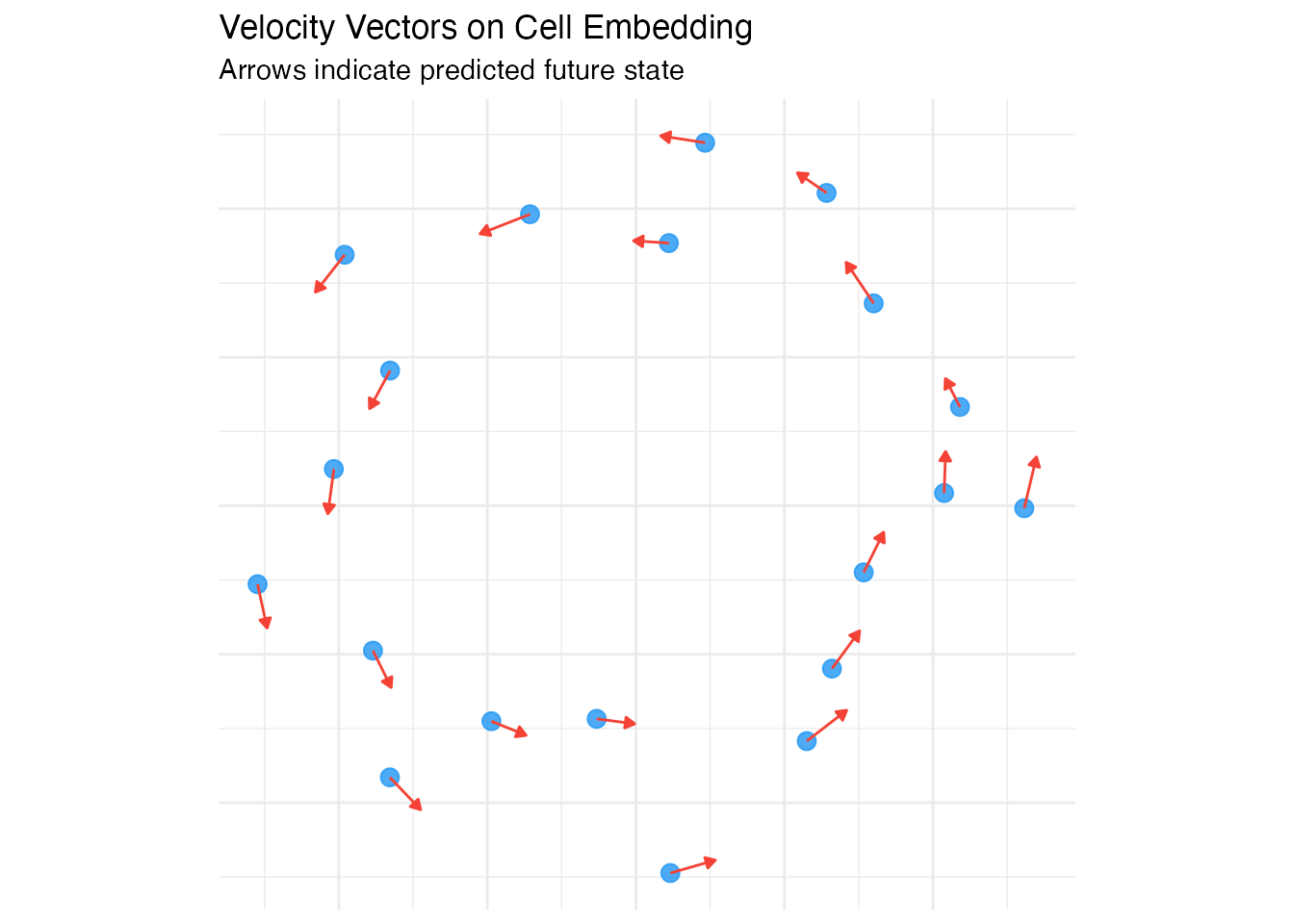
RNA velocity leverages the distinction between unspliced (nascent) and spliced (mature) mRNA to infer the direction and rate of gene expression changes.

The Kinetic Model

The dynamics of mRNA abundance can be described by a system of ordinary differential equations (ODEs):

$\frac{du}{dt} = \alpha(t) - \beta u$

$\frac{ds}{dt} = \beta u - \gamma s$

Where:

$u$ : unspliced mRNA abundance
$s$ : spliced mRNA abundance
$\alpha(t)$ : transcription rate (time-dependent)
$\beta$ : splicing rate (constitutive)
$\gamma$ : degradation rate (constitutive)

Analytical Solutions

Constant Transcription (Induction Phase)

When $\alpha(t) = \alpha$ (constant), the system has analytical solutions:

Unspliced mRNA: $u(t) = u_0 e^{-\beta t} + \frac{\alpha}{\beta}(1 - e^{-\beta t})$

Spliced mRNA: $s(t) = s_0 e^{-\gamma t} + \frac{\alpha}{\gamma}(1 - e^{-\gamma t}) + \frac{\alpha - u_0 \beta}{\gamma - \beta}(e^{-\gamma t} - e^{-\beta t})$

Zero Transcription (Repression Phase)

When transcription stops ( $\alpha = 0$ ):

$u(t) = u_0 e^{-\beta t}$

$s(t) = s_0 e^{-\gamma t} + \frac{\beta u_0}{\gamma - \beta}(e^{-\gamma t} - e^{-\beta t})$

Steady State

At equilibrium ( $du/dt = 0$ , $ds/dt = 0$ ):

$u_{ss} = \frac{\alpha}{\beta}$

$s_{ss} = \frac{\alpha}{\gamma}$

The ratio at steady state defines a fundamental relationship:

$\frac{u_{ss}}{s_{ss}} = \frac{\gamma}{\beta}$

Phase portrait showing the trajectory of gene expression during induction (blue) and repression (red) phases.

Velocity Estimation Models

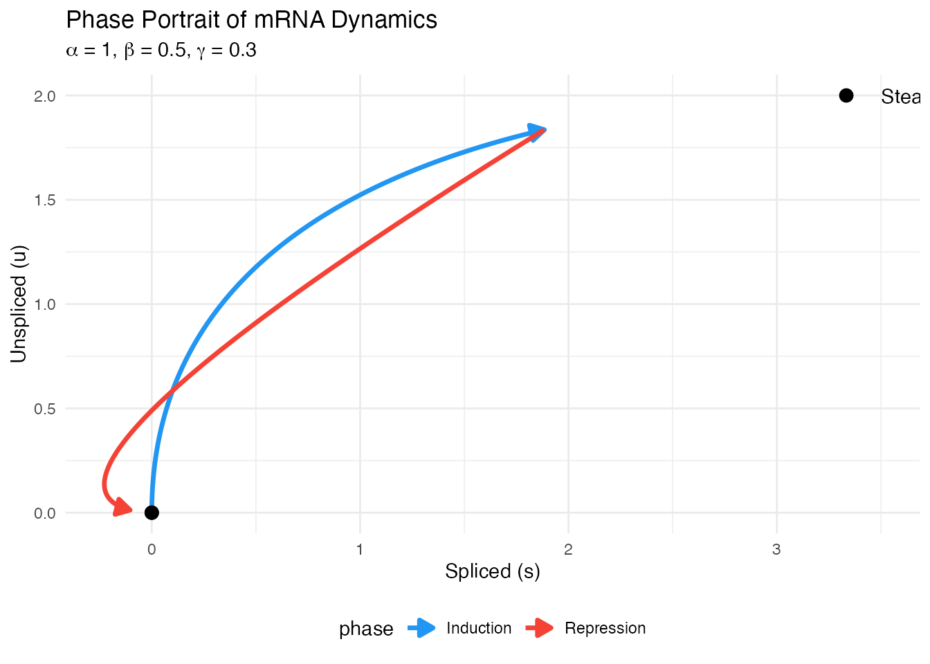
Model 1: Deterministic (Steady-State)

Assumption: Cells are near transcriptional steady state.

At steady state: $\gamma \approx \beta u / s$

Velocity: The deviation from steady state indicates the direction of change:

$v_s = \beta u - \gamma s$

If $v_s > 0$ : gene is being upregulated If $v_s < 0$ : gene is being downregulated

Implementation in scVeloR:

# Fit gamma by linear regression of u vs s
# v_s = β·u - γ·s = β(u - γ/β·s)
# Use regression: u ~ s to get slope γ/β

Model 2: Stochastic

Assumption: Account for transcriptional noise through second-order moments.

The stochastic model uses both first moments (mean expression) and second moments (variance, covariance):

$\text{Var}(u) = E[u^2] - E[u]^2$ $\text{Cov}(u,s) = E[us] - E[u]E[s]$

This provides more robust velocity estimates when transcriptional bursting is present.

Model 3: Dynamical

Assumption: Full kinetics model without steady-state assumption.

The dynamical model infers all kinetic parameters ( $\alpha$ , $\beta$ , $\gamma$ ) and the switching time ( $t_-$ ) using an Expectation-Maximization (EM) algorithm.

E-step: Assign latent time to each cell M-step: Update kinetic parameters

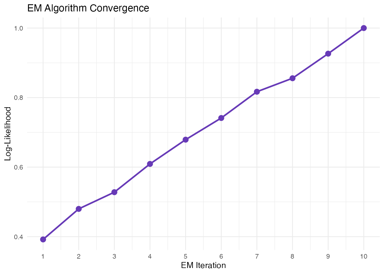
EM algorithm iteratively refines parameter estimates and time assignments.

Velocity Graph Construction

Cosine Similarity

The velocity graph captures cell-cell transitions based on velocity correlation:

$\text{cosine}(v_i, \delta_{ij}) = \frac{v_i \cdot \delta_{ij}}{||v_i|| \cdot ||\delta_{ij}||}$

Where: - $v_i$ : velocity vector for cell $i$ - $\delta_{ij}$ : expression difference between cell $i$ and $j$

Transition Probability

The transition probability from cell $i$ to cell $j$ :

$P_{ij} = \frac{\max(0, \text{cosine}(v_i, \delta_{ij}))}{\sum_k \max(0, \text{cosine}(v_i, \delta_{ik}))}$

Schematic of velocity-based transition probabilities.

Latent Time Inference

Gene-Shared Latent Time

The latent time represents the position of each cell along the differentiation trajectory:

$t_i = \frac{1}{|G|} \sum_{g \in G} t_{ig}$

Where $t_{ig}$ is the inferred time for cell $i$ based on gene $g$ .

Root Cell Identification

The root cells are identified as those with: 1. High connectivity in the velocity graph 2. Velocity vectors pointing “outward” (high end-point probability)

Model Selection Guidelines

Criterion	Steady-State	Stochastic	Dynamical
Speed	Fast	Medium	Slow
Data requirement	Low	Medium	High
Transcriptional dynamics	Equilibrium	Bursting	Transient
Parameter inference	γ only	γ only	α, β, γ, t_
Recommended use	Exploration	Default	Publication

References

Bergen, V., Lange, M., Peidli, S., Wolf, F. A., & Theis, F. J. (2020). Generalizing RNA velocity to transient cell states through dynamical modeling. Nature Biotechnology, 38, 1408–1414.
La Manno, G., Soldatov, R., Zeisel, A., et al. (2018). RNA velocity of single cells. Nature, 560, 494–498.
Svensson, V., & Pachter, L. (2018). RNA velocity: Molecular kinetics from single-cell RNA-seq. Molecular Cell, 72, 7–9.

Session Information

sessionInfo()
#> R version 4.4.0 (2024-04-24)
#> Platform: aarch64-apple-darwin20
#> Running under: macOS 15.6.1
#> 
#> Matrix products: default
#> BLAS:   /Library/Frameworks/R.framework/Versions/4.4-arm64/Resources/lib/libRblas.0.dylib 
#> LAPACK: /Library/Frameworks/R.framework/Versions/4.4-arm64/Resources/lib/libRlapack.dylib;  LAPACK version 3.12.0
#> 
#> locale:
#> [1] C
#> 
#> time zone: Asia/Shanghai
#> tzcode source: internal
#> 
#> attached base packages:
#> [1] stats     graphics  grDevices utils     datasets  methods   base     
#> 
#> other attached packages:
#> [1] ggplot2_4.0.1
#> 
#> loaded via a namespace (and not attached):
#>  [1] gtable_0.3.6       jsonlite_2.0.0     dplyr_1.1.4        compiler_4.4.0    
#>  [5] tidyselect_1.2.1   dichromat_2.0-0.1  jquerylib_0.1.4    systemfonts_1.3.1 
#>  [9] scales_1.4.0       textshaping_1.0.4  yaml_2.3.12        fastmap_1.2.0     
#> [13] R6_2.6.1           labeling_0.4.3     generics_0.1.4     knitr_1.51        
#> [17] htmlwidgets_1.6.4  tibble_3.3.1       desc_1.4.3         bslib_0.9.0       
#> [21] pillar_1.11.1      RColorBrewer_1.1-3 rlang_1.1.7        cachem_1.1.0      
#> [25] xfun_0.56          fs_1.6.6           sass_0.4.10        S7_0.2.1          
#> [29] otel_0.2.0         cli_3.6.5          pkgdown_2.1.3      withr_3.0.2       
#> [33] magrittr_2.0.4     digest_0.6.39      grid_4.4.0         lifecycle_1.0.5   
#> [37] vctrs_0.7.1        evaluate_1.0.5     glue_1.8.0         farver_2.1.2      
#> [41] ragg_1.5.0         rmarkdown_2.30     tools_4.4.0        pkgconfig_2.0.3   
#> [45] htmltools_0.5.9

Zaoqu Liu

2026-01-26