Performance Optimization Guide

Introduction

This guide provides strategies for optimizing scVeloR performance when working with large single-cell datasets. We cover memory management, parallel computing, and algorithmic optimizations.

Performance Architecture

scVeloR uses a hybrid architecture for optimal performance:

┌─────────────────────────────────────────────────────────────┐
│                    scVeloR Performance Stack                │
├─────────────────────────────────────────────────────────────┤
│  R Interface Layer                                          │
│    └── Vectorized R operations (Matrix package)            │
│    └── Parallel processing (future/parallel)               │
├─────────────────────────────────────────────────────────────┤
│  C++ Core (Rcpp/RcppArmadillo)                             │
│    └── Cosine similarity computation                        │
│    └── EM algorithm core                                    │
│    └── KNN computations                                     │
├─────────────────────────────────────────────────────────────┤
│  Sparse Matrix Support                                      │
│    └── Memory-efficient storage                             │
│    └── Optimized linear algebra                             │
└─────────────────────────────────────────────────────────────┘

Memory Optimization

Sparse Matrix Usage

scVeloR automatically uses sparse matrices when beneficial:

library(Matrix)

# Check sparsity of your data
sparsity <- sum(seurat_obj@assays$RNA@counts == 0) / 
            length(seurat_obj@assays$RNA@counts)
message(sprintf("Data sparsity: %.1f%%", sparsity * 100))

# Force sparse representation
seurat_obj@assays$RNA@counts <- as(seurat_obj@assays$RNA@counts, "dgCMatrix")

Memory Profiling

# Check memory usage
format(object.size(seurat_obj), units = "GB")

# Monitor during analysis
gc()  # Garbage collection
memory.size()  # Current memory usage (Windows)
pryr::mem_used()  # Cross-platform

Chunked Processing

For very large datasets, process in chunks:

# Split cells into chunks
n_cells <- ncol(seurat_obj)
chunk_size <- 10000
n_chunks <- ceiling(n_cells / chunk_size)

# Process each chunk
results <- list()
for (i in seq_len(n_chunks)) {
  start_idx <- (i - 1) * chunk_size + 1
  end_idx <- min(i * chunk_size, n_cells)
  
  chunk_obj <- seurat_obj[, start_idx:end_idx]
  results[[i]] <- process_velocity_chunk(chunk_obj)
  
  gc()  # Clean up after each chunk
}

# Merge results
final_results <- merge_velocity_results(results)

Parallel Computing

Using the future Package

library(future)
library(future.apply)

# Check available cores
availableCores()

# Setup parallel backend
plan(multisession, workers = 4)  # 4 parallel workers

# Run velocity analysis
seurat_obj <- run_velocity(seurat_obj, 
                           mode = "dynamical",
                           n_cores = 4)

# Reset to sequential
plan(sequential)

Platform-Specific Configuration

# Detect OS and configure
if (.Platform$OS.type == "unix") {
  # Unix/Mac: use multicore for shared memory
  plan(multicore, workers = availableCores() - 1)
} else {
  # Windows: use multisession (separate R processes)
  plan(multisession, workers = availableCores() - 1)
}

Parallel Best Practices

Scenario	Recommended Setup
< 10K cells	Sequential (overhead > benefit)
10K - 50K cells	4 workers
50K - 100K cells	8 workers
> 100K cells	Max available - 1

# Automatic configuration based on dataset size
n_cells <- ncol(seurat_obj)

if (n_cells < 10000) {
  n_workers <- 1
} else if (n_cells < 50000) {
  n_workers <- min(4, availableCores() - 1)
} else {
  n_workers <- availableCores() - 1
}

if (n_workers > 1) {
  plan(multisession, workers = n_workers)
}

Algorithmic Optimizations

Gene Selection

Reducing the number of genes dramatically speeds up computation:

# Use fewer genes for speed
seurat_obj <- velocity(seurat_obj, 
                       mode = "dynamical",
                       n_top_genes = 1000)  # Default: 2000

# Or use highly variable genes
hvg <- Seurat::VariableFeatures(seurat_obj)
seurat_obj <- velocity(seurat_obj,
                       mode = "dynamical", 
                       genes = hvg[1:500])  # Top 500 HVGs

Neighbor Graph Approximation

For large datasets, use approximate nearest neighbor algorithms:

# Exact KNN (default, slower for large data)
seurat_obj <- compute_neighbors(seurat_obj, 
                                 n_neighbors = 30,
                                 method = "exact")

# Approximate KNN with Annoy (faster)
seurat_obj <- compute_neighbors(seurat_obj,
                                 n_neighbors = 30,
                                 method = "annoy",
                                 n_trees = 50)

# Approximate KNN with HNSW (fastest for very large data)
seurat_obj <- compute_neighbors(seurat_obj,
                                 n_neighbors = 30,
                                 method = "hnsw",
                                 M = 16, ef = 200)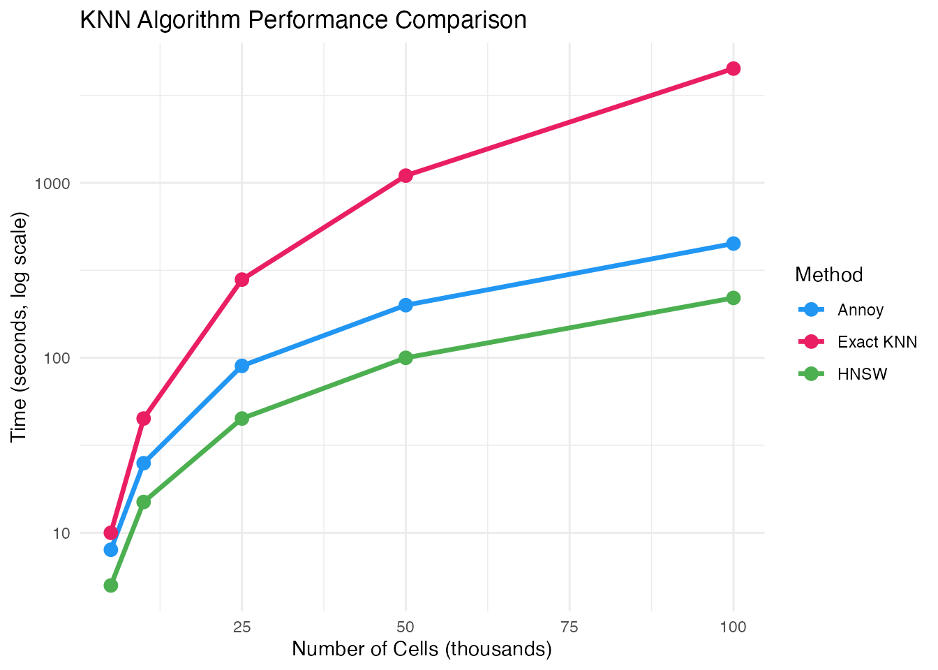

Benchmark Comparison

Computational time for different methods and dataset sizes.

EM Algorithm Optimization

# Fewer iterations for faster (less accurate) results
seurat_obj <- recover_dynamics(seurat_obj, max_iter = 5)

# More iterations for better accuracy
seurat_obj <- recover_dynamics(seurat_obj, max_iter = 20)

# Early stopping based on convergence
seurat_obj <- recover_dynamics(seurat_obj, 
                                max_iter = 20,
                                tol = 1e-4)  # Stop if change < tol

Hardware Recommendations

Memory Requirements

Dataset Size	Recommended RAM
< 10K cells	8 GB
10K - 50K cells	16 GB
50K - 100K cells	32 GB
> 100K cells	64+ GB

Compute Requirements

Analysis Type	CPU Cores	Time Estimate (50K cells)
Steady-state	1	~2 min
Stochastic	4	~10 min
Dynamical	8	~45 min

Profiling Your Analysis

Timing Code Blocks

library(tictoc)

# Profile each step
tic("Total analysis")

tic("Preprocessing")
seurat_obj <- prepare_velocity(seurat_obj)
toc()

tic("Velocity computation")
seurat_obj <- velocity(seurat_obj, mode = "dynamical")
toc()

tic("Velocity graph")
seurat_obj <- velocity_graph(seurat_obj)
toc()

toc()  # Total

Identifying Bottlenecks

# Use Rprof for detailed profiling
Rprof("velocity_profile.out")
seurat_obj <- velocity(seurat_obj, mode = "dynamical")
Rprof(NULL)

# Analyze results
summaryRprof("velocity_profile.out")

Practical Workflow for Large Data

Optimized Pipeline

library(scVeloR)
library(future)

# 1. Configure parallel backend
n_cores <- min(8, availableCores() - 1)
plan(multisession, workers = n_cores)

# 2. Use sparse matrices
seurat_obj@assays$RNA@counts <- as(
  seurat_obj@assays$RNA@counts, "dgCMatrix"
)

# 3. Preprocessing with filtering
seurat_obj <- prepare_velocity(
  seurat_obj,
  min_counts = 30,     # Stricter filtering
  min_cells = 50,
  n_neighbors = 30
)

# 4. Use approximate KNN
seurat_obj <- compute_neighbors(
  seurat_obj,
  method = "hnsw",
  n_neighbors = 30
)

# 5. Velocity with fewer genes
seurat_obj <- velocity(
  seurat_obj,
  mode = "dynamical",
  n_top_genes = 1000,  # Reduced from 2000
  max_iter = 8,        # Reduced from 10
  n_cores = n_cores
)

# 6. Build velocity graph
seurat_obj <- velocity_graph(
  seurat_obj,
  n_neighbors = 30,
  n_cores = n_cores
)

# 7. Reset backend
plan(sequential)
gc()

Memory-Efficient Visualization

# Subsample for visualization
set.seed(42)
sample_idx <- sample(ncol(seurat_obj), min(5000, ncol(seurat_obj)))

# Create subsampled plot
p <- plot_velocity(seurat_obj[, sample_idx], 
                   embedding = "umap",
                   n_arrows = 500)

# Save to file instead of displaying
ggsave("velocity_plot.pdf", p, width = 8, height = 6)

Troubleshooting Performance Issues

Common Issues and Solutions

Issue	Cause	Solution
Out of memory	Dense matrices	Use sparse matrices
Slow KNN	Large dataset	Use HNSW
Long EM runtime	Too many genes	Reduce n_top_genes
Worker errors	Memory per worker	Reduce workers or increase RAM

Quick Diagnostics

# System info
Sys.info()
.Machine$sizeof.pointer  # 4 = 32-bit, 8 = 64-bit

# R memory limit (Windows)
memory.limit()

# Check for data issues
sum(is.na(seurat_obj@misc$scVeloR$Ms))  # NA values
range(seurat_obj@misc$scVeloR$Ms)       # Value ranges

Summary

Key optimization strategies:

Memory: Use sparse matrices, chunk processing for very large data
Parallelization: Use future package with appropriate workers
Algorithms: Use approximate KNN (HNSW) for large datasets
Parameters: Reduce genes and EM iterations for speed

Session Information

sessionInfo()
#> R version 4.4.0 (2024-04-24)
#> Platform: aarch64-apple-darwin20
#> Running under: macOS 15.6.1
#> 
#> Matrix products: default
#> BLAS:   /Library/Frameworks/R.framework/Versions/4.4-arm64/Resources/lib/libRblas.0.dylib 
#> LAPACK: /Library/Frameworks/R.framework/Versions/4.4-arm64/Resources/lib/libRlapack.dylib;  LAPACK version 3.12.0
#> 
#> locale:
#> [1] C
#> 
#> time zone: Asia/Shanghai
#> tzcode source: internal
#> 
#> attached base packages:
#> [1] stats     graphics  grDevices utils     datasets  methods   base     
#> 
#> other attached packages:
#> [1] ggplot2_4.0.1
#> 
#> loaded via a namespace (and not attached):
#>  [1] gtable_0.3.6       jsonlite_2.0.0     dplyr_1.1.4        compiler_4.4.0    
#>  [5] tidyselect_1.2.1   dichromat_2.0-0.1  jquerylib_0.1.4    systemfonts_1.3.1 
#>  [9] scales_1.4.0       textshaping_1.0.4  yaml_2.3.12        fastmap_1.2.0     
#> [13] R6_2.6.1           labeling_0.4.3     generics_0.1.4     knitr_1.51        
#> [17] htmlwidgets_1.6.4  tibble_3.3.1       desc_1.4.3         bslib_0.9.0       
#> [21] pillar_1.11.1      RColorBrewer_1.1-3 rlang_1.1.7        cachem_1.1.0      
#> [25] xfun_0.56          fs_1.6.6           sass_0.4.10        S7_0.2.1          
#> [29] otel_0.2.0         cli_3.6.5          pkgdown_2.1.3      withr_3.0.2       
#> [33] magrittr_2.0.4     digest_0.6.39      grid_4.4.0         lifecycle_1.0.5   
#> [37] vctrs_0.7.1        evaluate_1.0.5     glue_1.8.0         farver_2.1.2      
#> [41] ragg_1.5.0         rmarkdown_2.30     tools_4.4.0        pkgconfig_2.0.3   
#> [45] htmltools_0.5.9

Zaoqu Liu

2026-01-26