Dynamical Model Deep Dive

Introduction

The dynamical model in scVeloR represents the most sophisticated approach to RNA velocity estimation. Unlike simpler steady-state methods, it infers the full kinetic parameters of gene expression without assuming transcriptional equilibrium.

This vignette provides a comprehensive guide to:

Understanding the underlying mathematics
Implementing the dynamical model
Interpreting results
Troubleshooting common issues

Mathematical Foundation

The Transcriptional Switch Model

The dynamical model assumes genes undergo a transcriptional switch:

Induction phase ( $t < t_-$ ): Transcription is active ( $\alpha > 0$ )
Repression phase ( $t \geq t_-$ ): Transcription stops ( $\alpha = 0$ )

ODE System

Induction phase ( $t < t_-$ ): $\frac{du}{dt} = \alpha - \beta u$ $\frac{ds}{dt} = \beta u - \gamma s$

Repression phase ( $t \geq t_-$ ): $\frac{du}{dt} = -\beta u$ $\frac{ds}{dt} = \beta u - \gamma s$

Analytical Solutions

Induction phase: $u(t) = u_0 e^{-\beta t} + \frac{\alpha}{\beta}(1 - e^{-\beta t})$ $s(t) = s_0 e^{-\gamma t} + \frac{\alpha}{\gamma}(1 - e^{-\gamma t}) + \frac{\alpha - u_0\beta}{\gamma - \beta}(e^{-\gamma t} - e^{-\beta t})$

Repression phase (starting from $u_-, s_-$ at $t_-$ ): $u(t) = u_- e^{-\beta(t-t_-)}$ $s(t) = s_- e^{-\gamma(t-t_-)} + \frac{\beta u_-}{\gamma - \beta}(e^{-\gamma(t-t_-)} - e^{-\beta(t-t_-)})$

Gene expression trajectory showing induction and repression phases.

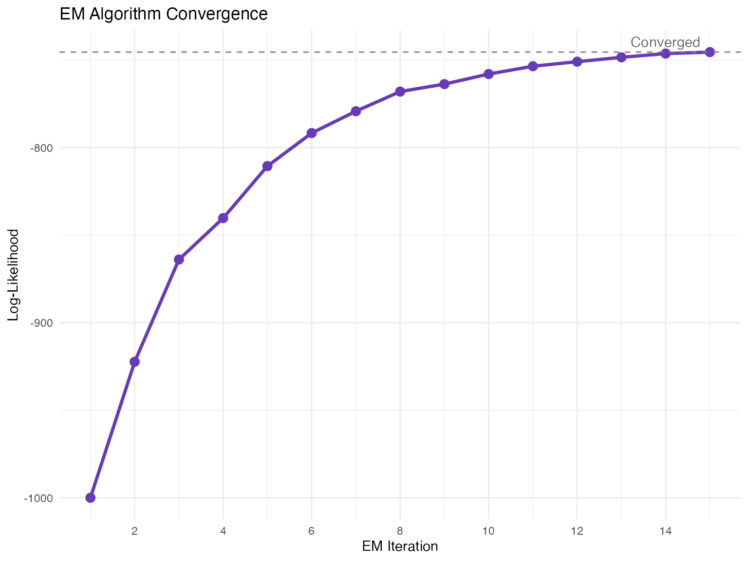
The EM Algorithm

Overview

The dynamical model uses an Expectation-Maximization (EM) algorithm to jointly infer:

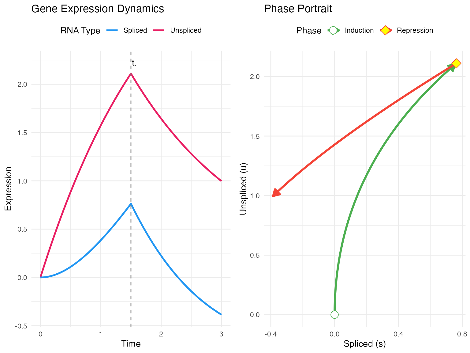
Kinetic parameters: $\alpha$ , $\beta$ , $\gamma$ for each gene
Switching time: $t_-$ for each gene
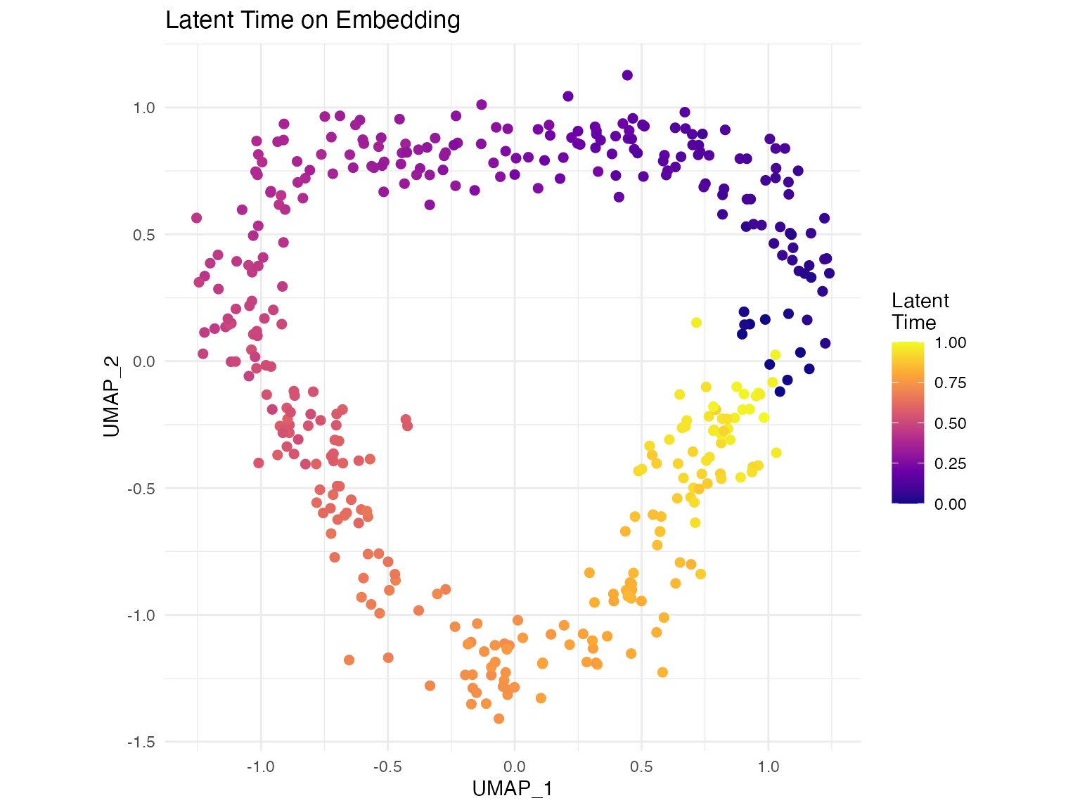
Latent time: $t_i$ for each cell

E-Step: Time Assignment

Given current parameter estimates, assign latent time to each cell by minimizing the residual:

$t_i = \arg\min_t \left( (u_i - \hat{u}(t))^2 + (s_i - \hat{s}(t))^2 \right)$

M-Step: Parameter Update

Given time assignments, update parameters by maximum likelihood:

$(\hat{\alpha}, \hat{\beta}, \hat{\gamma}, \hat{t}_-) = \arg\max \sum_i \log P(u_i, s_i | \alpha, \beta, \gamma, t_-, t_i)$

EM algorithm convergence showing iterative improvement.

Implementation in scVeloR

Basic Usage

library(scVeloR)

# Run dynamical model
seurat_obj <- velocity(seurat_obj, 
                       mode = "dynamical",
                       max_iter = 10)

Step-by-Step Approach

# Step 1: Identify velocity genes using steady-state
seurat_obj <- velocity(seurat_obj, mode = "deterministic")

# Step 2: Recover full dynamics
seurat_obj <- recover_dynamics(
  seurat_obj,
  genes = "velocity_genes",  # Use pre-selected genes
  n_top_genes = 2000,        # Or top N by variance
  max_iter = 10,             # EM iterations
  fit_scaling = TRUE,        # Estimate scaling factor
  n_cores = 4                # Parallel processing
)

# Step 3: Compute velocity from dynamics
seurat_obj <- velocity_from_dynamics(seurat_obj)

# Step 4: Compute latent time
seurat_obj <- compute_latent_time(seurat_obj)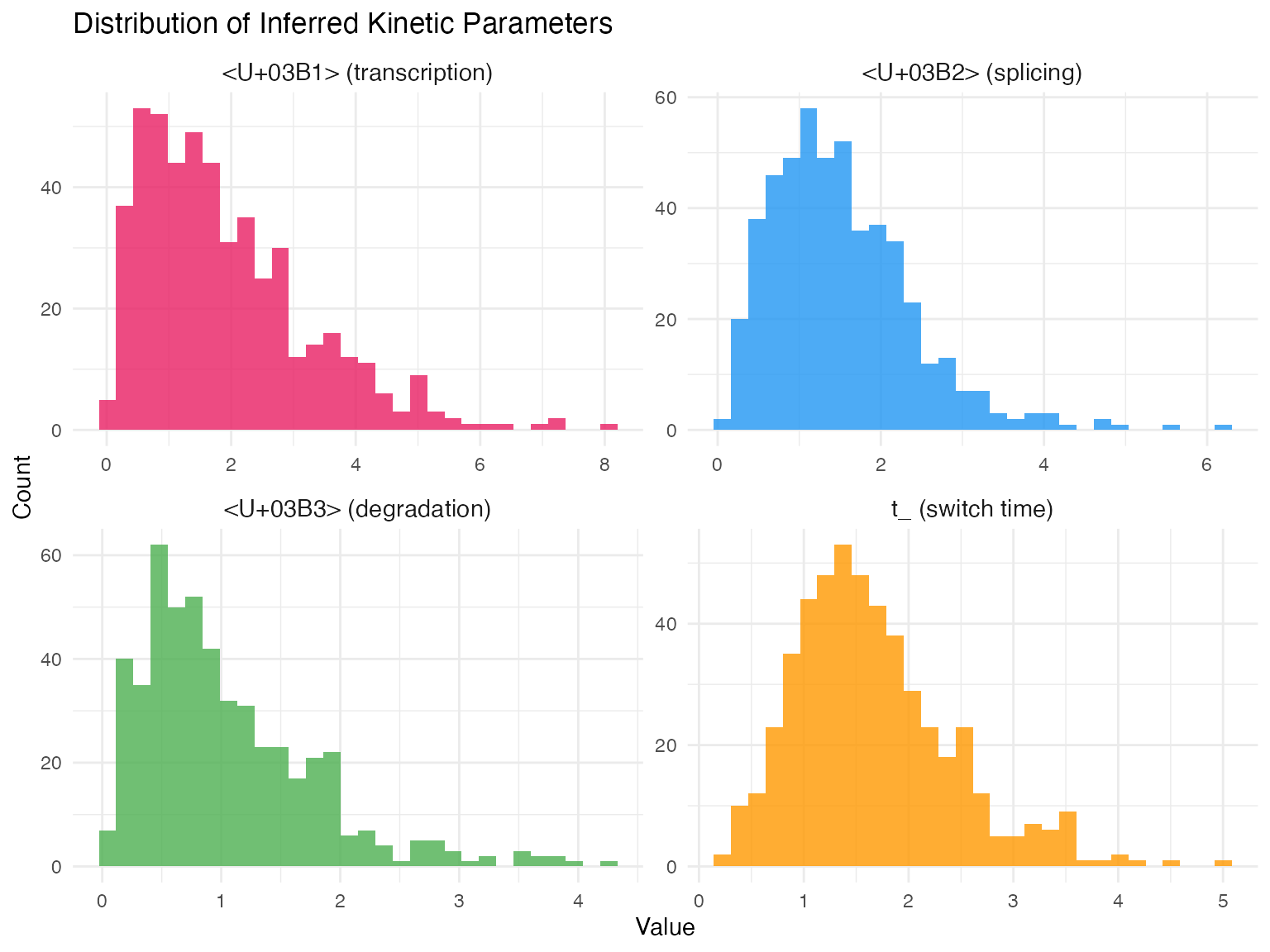

Parameter Details

Parameter	Default	Description
`max_iter`	10	Maximum EM iterations
`n_top_genes`	2000	Number of top variable genes
`fit_scaling`	TRUE	Estimate u/s scaling factor
`t_max`	20	Maximum allowed latent time
`min_likelihood`	0.1	Minimum gene likelihood threshold

Interpreting Results

Kinetic Parameters

Distribution of inferred kinetic parameters across genes.

Latent Time

Latent time projected onto embedding showing differentiation trajectory.

Quality Control

Gene Fit Quality

# Check gene fit quality
gene_params <- seurat_obj@misc$scVeloR$dynamics$gene_params

# High-quality genes have high likelihood
good_genes <- gene_params[gene_params$likelihood > 0.3, ]
print(head(good_genes))

# Visualize fit for specific gene
plot_phase(seurat_obj, gene = "Sox2", show_fit = TRUE)

Convergence Check

# Check if EM converged
dynamics <- seurat_obj@misc$scVeloR$dynamics

# Likelihood should increase with iterations
if (!is.null(dynamics$likelihood_trace)) {
  plot(dynamics$likelihood_trace, type = "l",
       xlab = "Iteration", ylab = "Log-Likelihood",
       main = "EM Convergence")
}

Velocity Confidence

# Compute velocity confidence
seurat_obj <- velocity_confidence(seurat_obj)

# Check distribution
hist(seurat_obj$velocity_confidence, breaks = 50,
     main = "Velocity Confidence Distribution",
     xlab = "Confidence Score")

Troubleshooting

Common Issues

Poor convergence
- Increase max_iter
- Filter low-quality genes
- Check data normalization
Unrealistic parameter estimates
- Check for outlier cells
- Verify spliced/unspliced layer quality
- Try different gene selection
Inconsistent latent time
- Use more genes for averaging
- Filter genes with low likelihood
- Check for batch effects

Best Practices

# 1. Pre-filter low-quality data
seurat_obj <- prepare_velocity(seurat_obj,
                                min_counts = 20,
                                min_cells = 30)

# 2. Use sufficient EM iterations
seurat_obj <- velocity(seurat_obj, 
                       mode = "dynamical",
                       max_iter = 15)  # More iterations

# 3. Check results
velocity_summary(seurat_obj)

# 4. Filter by gene quality
gene_params <- seurat_obj@misc$scVeloR$dynamics$gene_params
good_fit <- gene_params$likelihood > 0.2
message(sprintf("%d / %d genes with good fit", sum(good_fit), length(good_fit)))

Advanced Topics

Scaling Factor

The scaling factor accounts for differences in capture efficiency between spliced and unspliced molecules:

$u_{observed} = \text{scaling} \times u_{true}$

Effect of scaling factor on phase portrait alignment.

Parallel Processing

# Use multiple cores for large datasets
library(future)
plan(multisession, workers = 8)

seurat_obj <- velocity(seurat_obj, 
                       mode = "dynamical",
                       n_cores = 8)

plan(sequential)  # Reset

Summary

The dynamical model provides the most comprehensive RNA velocity analysis by:

Inferring full kinetics: α, β, γ for each gene
Handling transient states: No equilibrium assumption
Providing latent time: Absolute temporal ordering of cells

Use it when you need: - Publication-quality results - Analysis of rapidly changing processes - Interpretation of kinetic parameters - Latent time for downstream analysis

Session Information

sessionInfo()
#> R version 4.4.0 (2024-04-24)
#> Platform: aarch64-apple-darwin20
#> Running under: macOS 15.6.1
#> 
#> Matrix products: default
#> BLAS:   /Library/Frameworks/R.framework/Versions/4.4-arm64/Resources/lib/libRblas.0.dylib 
#> LAPACK: /Library/Frameworks/R.framework/Versions/4.4-arm64/Resources/lib/libRlapack.dylib;  LAPACK version 3.12.0
#> 
#> locale:
#> [1] C
#> 
#> time zone: Asia/Shanghai
#> tzcode source: internal
#> 
#> attached base packages:
#> [1] stats     graphics  grDevices utils     datasets  methods   base     
#> 
#> other attached packages:
#> [1] tidyr_1.3.2   gridExtra_2.3 ggplot2_4.0.1
#> 
#> loaded via a namespace (and not attached):
#>  [1] gtable_0.3.6       jsonlite_2.0.0     dplyr_1.1.4        compiler_4.4.0    
#>  [5] tidyselect_1.2.1   dichromat_2.0-0.1  jquerylib_0.1.4    systemfonts_1.3.1 
#>  [9] scales_1.4.0       textshaping_1.0.4  yaml_2.3.12        fastmap_1.2.0     
#> [13] R6_2.6.1           labeling_0.4.3     generics_0.1.4     knitr_1.51        
#> [17] htmlwidgets_1.6.4  tibble_3.3.1       desc_1.4.3         bslib_0.9.0       
#> [21] pillar_1.11.1      RColorBrewer_1.1-3 rlang_1.1.7        cachem_1.1.0      
#> [25] xfun_0.56          fs_1.6.6           sass_0.4.10        S7_0.2.1          
#> [29] otel_0.2.0         viridisLite_0.4.2  cli_3.6.5          pkgdown_2.1.3     
#> [33] withr_3.0.2        magrittr_2.0.4     digest_0.6.39      grid_4.4.0        
#> [37] lifecycle_1.0.5    vctrs_0.7.1        evaluate_1.0.5     glue_1.8.0        
#> [41] farver_2.1.2       ragg_1.5.0         purrr_1.2.1        rmarkdown_2.30    
#> [45] tools_4.4.0        pkgconfig_2.0.3    htmltools_0.5.9

Zaoqu Liu

2026-01-26