Velocity Model Comparison

Introduction

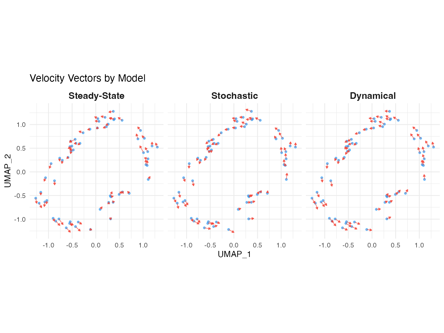
scVeloR implements three velocity estimation models, each with distinct assumptions and use cases. This vignette provides a comprehensive comparison to help you choose the appropriate model for your data.

Model Overview

1. Deterministic (Steady-State) Model

Assumption: Cells are near transcriptional equilibrium.

Key equation: $\gamma \approx \frac{\beta u}{s}$

Velocity: $v_s = \beta u - \gamma s$

Pros: - Fast computation - Requires minimal data - Works well for slowly changing processes

Cons: - May miss transient dynamics - Assumes equilibrium

2. Stochastic Model

Assumption: Accounts for transcriptional bursting and noise.

Uses: First and second-order moments (mean, variance, covariance)

Pros: - More robust to noise - Better for bursty transcription - Intermediate computational cost

Cons: - Still assumes near-equilibrium - Requires sufficient cell numbers

3. Dynamical Model

Assumption: Full kinetics without equilibrium constraint.

Inferred parameters: α (transcription), β (splicing), γ (degradation), t_ (switching time)

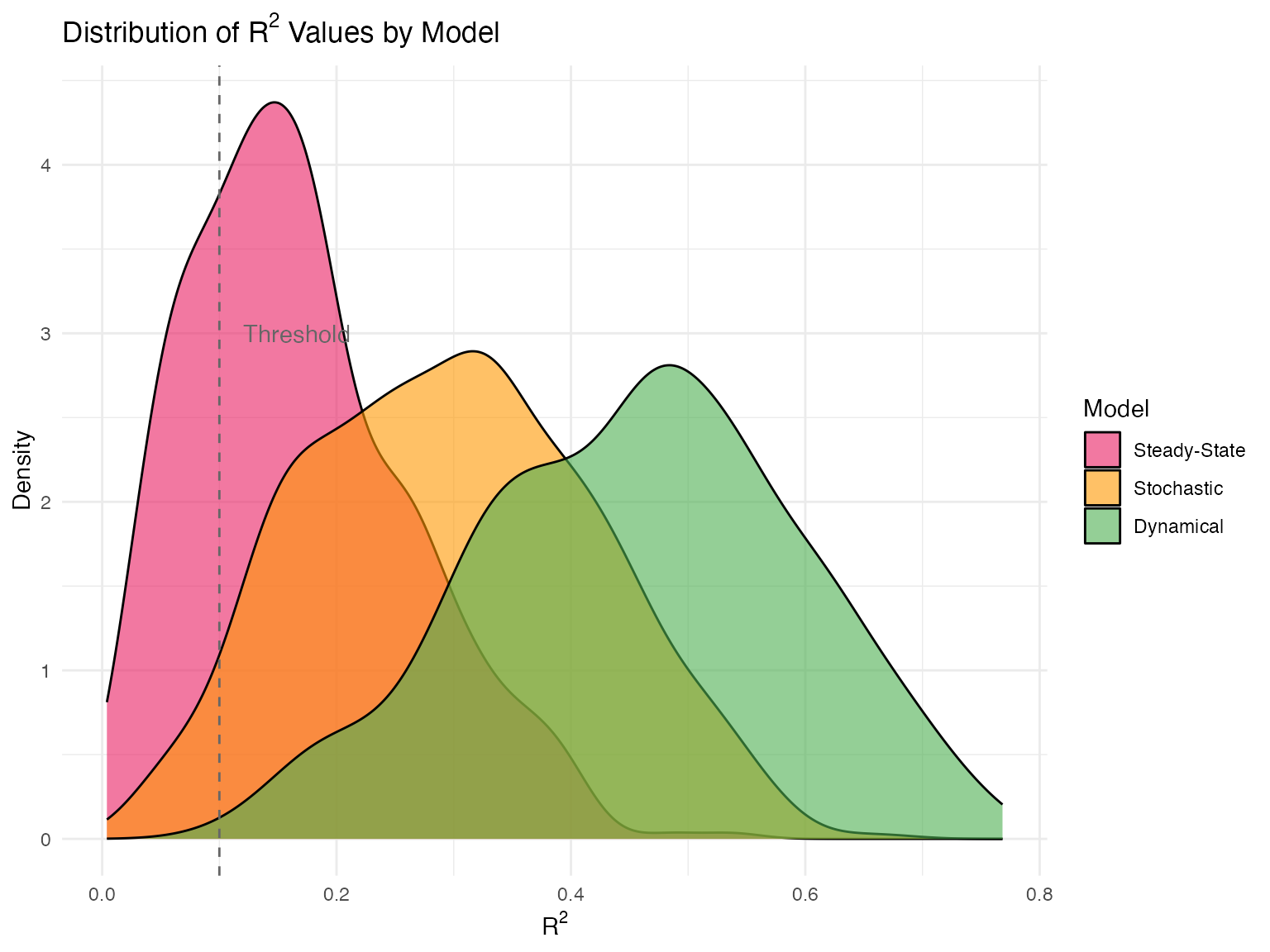
Pros: - Captures transient states - Infers absolute time - Most accurate for complex dynamics

Cons: - Computationally intensive - Requires high-quality data - May overfit small datasets

Comparison Table

Feature	Steady-State	Stochastic	Dynamical
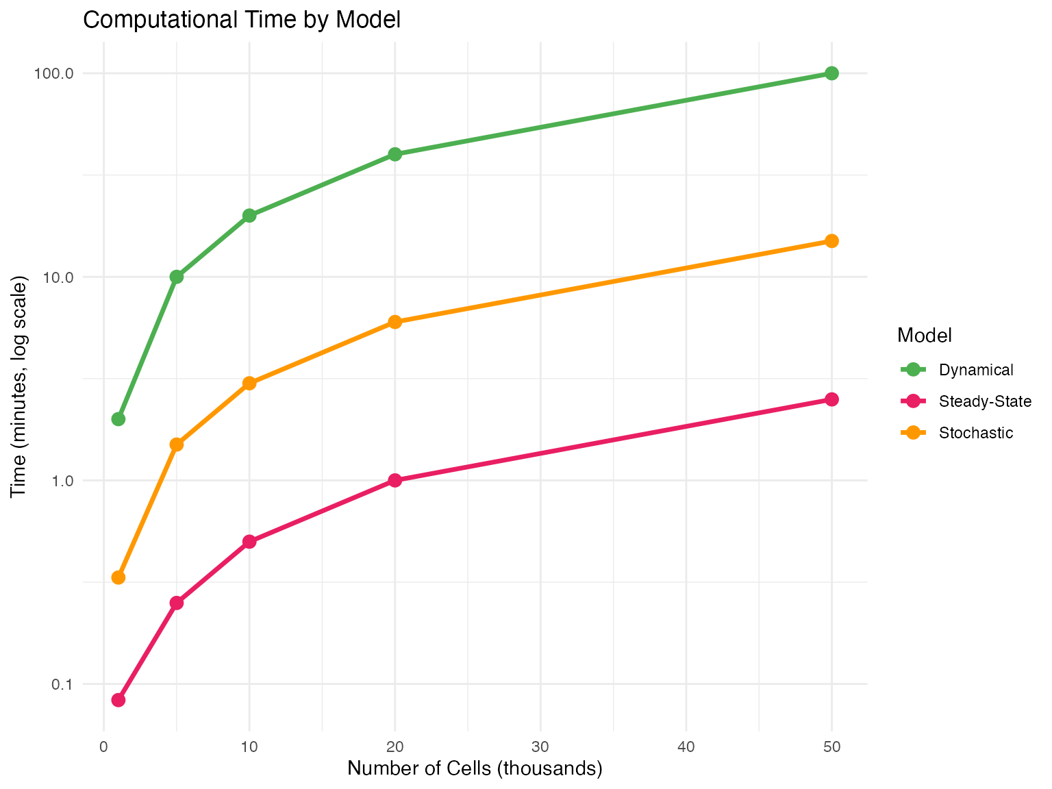
Speed	~1 min	~5 min	~30 min
Data requirement	Low	Medium	High
Parameters inferred	<U+03B3> only	<U+03B3> only	<U+03B1>, <U+03B2>, <U+03B3>, t_
Handles transient states	No	Partial	Yes
Provides latent time	No	No	Yes
Recommended dataset size	>1,000 cells	>3,000 cells	>5,000 cells
Best for	Exploration	Default choice	Publication

Visual Comparison

Velocity vectors from different models showing varying sensitivity to dynamics.

When to Use Each Model

Use Steady-State When:

Quick exploration: Getting a first look at your data
Large datasets: >50,000 cells where speed matters
Equilibrium processes: Homeostatic cell populations
Limited compute resources

seurat_obj <- velocity(seurat_obj, mode = "deterministic")

Use Stochastic When:

Default choice: Good balance of speed and accuracy
Noisy data: High technical variability
Transcriptional bursting: Known bursty gene expression

seurat_obj <- velocity(seurat_obj, mode = "stochastic")

Use Dynamical When:

Publication-quality results: Need the most accurate estimates
Transient states: Rapid differentiation, cell activation
Latent time needed: Want absolute temporal ordering
Parameter interpretation: Need kinetic rate estimates

seurat_obj <- velocity(seurat_obj, mode = "dynamical", max_iter = 10)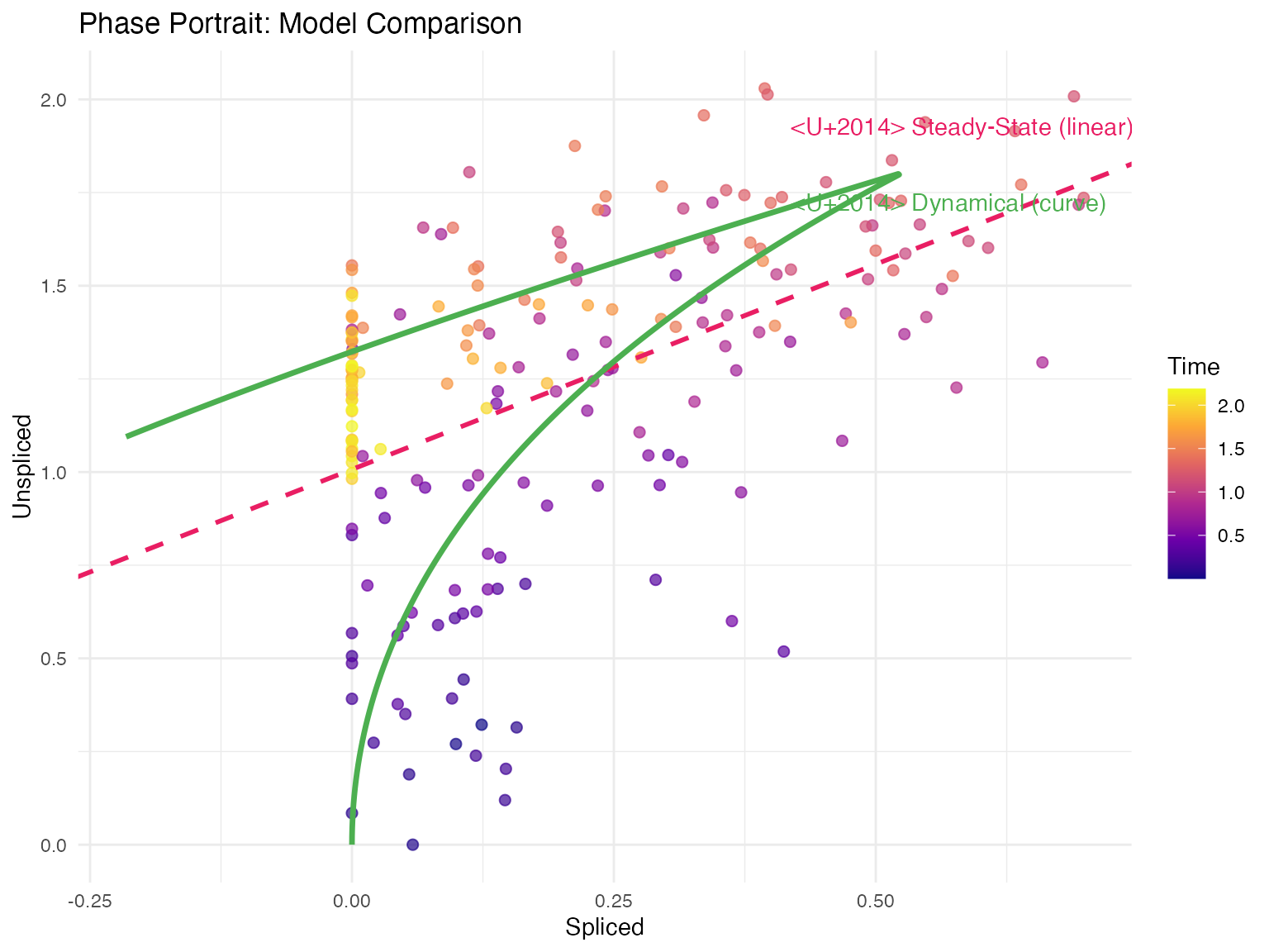

Diagnostic Plots

Phase Portrait Comparison

Phase portraits showing how each model fits the data.

R-squared Distribution

Distribution of R<U+00B2> values indicating model fit quality.

Computational Benchmarks

Computational time comparison across dataset sizes.

Practical Workflow

Recommended Approach

library(scVeloR)

# 1. Start with steady-state for quick exploration
seurat_obj <- velocity(seurat_obj, mode = "deterministic")
plot_velocity(seurat_obj)

# 2. If results look promising, try stochastic
seurat_obj <- velocity(seurat_obj, mode = "stochastic")
plot_velocity(seurat_obj)

# 3. For final analysis, use dynamical
seurat_obj <- velocity(seurat_obj, mode = "dynamical")
plot_velocity(seurat_obj)

# 4. Compare results
velocity_summary(seurat_obj)

Session Information

sessionInfo()
#> R version 4.4.0 (2024-04-24)
#> Platform: aarch64-apple-darwin20
#> Running under: macOS 15.6.1
#> 
#> Matrix products: default
#> BLAS:   /Library/Frameworks/R.framework/Versions/4.4-arm64/Resources/lib/libRblas.0.dylib 
#> LAPACK: /Library/Frameworks/R.framework/Versions/4.4-arm64/Resources/lib/libRlapack.dylib;  LAPACK version 3.12.0
#> 
#> locale:
#> [1] C
#> 
#> time zone: Asia/Shanghai
#> tzcode source: internal
#> 
#> attached base packages:
#> [1] stats     graphics  grDevices utils     datasets  methods   base     
#> 
#> other attached packages:
#> [1] ggplot2_4.0.1
#> 
#> loaded via a namespace (and not attached):
#>  [1] gtable_0.3.6       jsonlite_2.0.0     dplyr_1.1.4        compiler_4.4.0    
#>  [5] tidyselect_1.2.1   dichromat_2.0-0.1  jquerylib_0.1.4    systemfonts_1.3.1 
#>  [9] scales_1.4.0       textshaping_1.0.4  yaml_2.3.12        fastmap_1.2.0     
#> [13] R6_2.6.1           labeling_0.4.3     generics_0.1.4     knitr_1.51        
#> [17] htmlwidgets_1.6.4  tibble_3.3.1       desc_1.4.3         bslib_0.9.0       
#> [21] pillar_1.11.1      RColorBrewer_1.1-3 rlang_1.1.7        cachem_1.1.0      
#> [25] xfun_0.56          fs_1.6.6           sass_0.4.10        S7_0.2.1          
#> [29] otel_0.2.0         viridisLite_0.4.2  cli_3.6.5          pkgdown_2.1.3     
#> [33] withr_3.0.2        magrittr_2.0.4     digest_0.6.39      grid_4.4.0        
#> [37] lifecycle_1.0.5    vctrs_0.7.1        evaluate_1.0.5     glue_1.8.0        
#> [41] farver_2.1.2       ragg_1.5.0         rmarkdown_2.30     tools_4.4.0       
#> [45] pkgconfig_2.0.3    htmltools_0.5.9

Zaoqu Liu

2026-01-26