GRN Inference Details

Overview

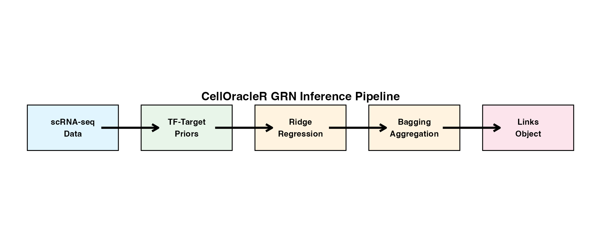
Gene Regulatory Network (GRN) inference is the foundation of CellOracleR analysis. This vignette provides detailed documentation of the GRN inference pipeline.

Pipeline Architecture

Step 1: Input Data Preparation

Expression Matrix

CellOracleR requires a normalized expression matrix (genes × cells):

# From Seurat object
library(Seurat)
library(CellOracleR)

# Create Oracle object
oracle <- create_oracle(
  seurat_obj,
  cluster_col = "seurat_clusters",
  embedding_name = "umap"
)

# Extract expression data
expr_matrix <- oracle$get_expression()
dim(expr_matrix)  # genes × cells

Recommendations:

Use normalized data (log-transformed)
Filter low-quality cells and genes
2,000-5,000 highly variable genes typically sufficient

TF-Target Prior Dictionary

The TF-target dictionary specifies which TFs can potentially regulate each gene:

# Structure: list with gene names as keys
# Each element contains a character vector of potential TF regulators

TFdict <- list(
  Gene1 = c("TF_A", "TF_B", "TF_C"),
  Gene2 = c("TF_A", "TF_D"),
  Gene3 = c("TF_B", "TF_C", "TF_D", "TF_E")
)

Sources for TF-target priors:

Motif analysis (recommended): Scan promoter sequences for TF binding motifs
ChIP-seq data: Experimentally determined TF binding sites
Literature curation: Known regulatory relationships
ATAC-seq + Cicero: Accessibility-based predictions

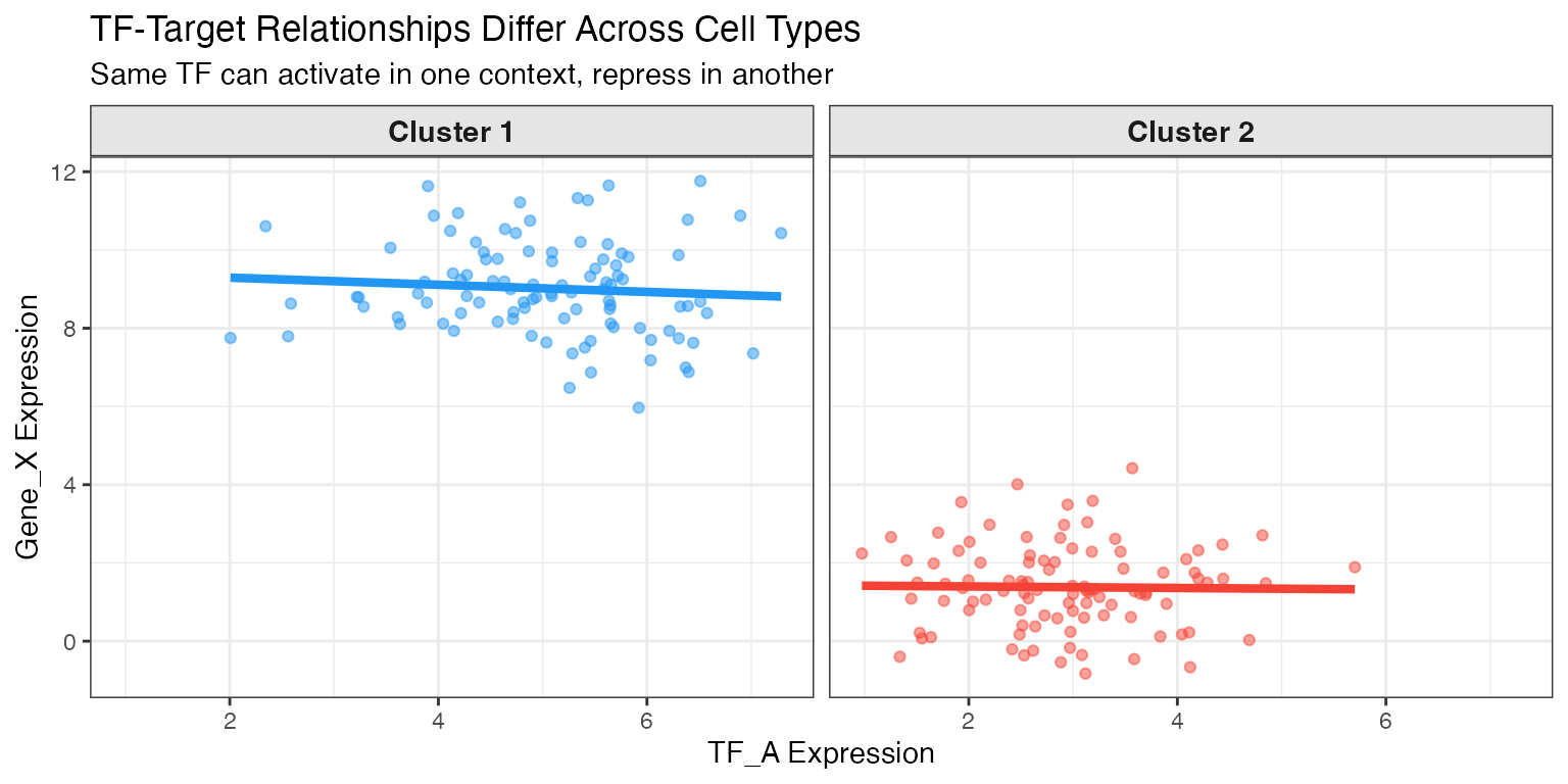
Step 2: Cluster-Specific GRN Fitting

GRNs are fitted separately for each cell cluster to capture cell-type-specific regulatory logic.

Per-Cluster Fitting

# Fit GRN for specific cluster
oracle$fit_grn_for_simulation(
  GRN_unit = "cluster",          # Group by cluster
  alpha = 10,                     # Regularization strength
  bagging_number = 200,           # Number of bootstrap iterations
  use_cache = TRUE                # Cache intermediate results
)

Why cluster-specific?

Step 3: Ridge Regression Details

Regularization Parameter (α)

The regularization parameter controls the bias-variance trade-off:

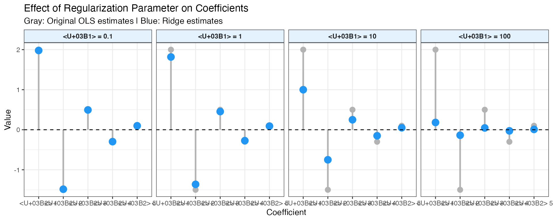
Guidelines for choosing α:

α value	Effect	Use case
0.1-1	Minimal shrinkage	High-quality data, few predictors
1-10	Moderate shrinkage	Standard scRNA-seq (recommended)
10-100	Strong shrinkage	Noisy data, many predictors
>100	Heavy shrinkage	Highly correlated predictors

Default: α = 10 - provides good balance for typical scRNA-seq data.

Handling Zero Variance

When a gene has zero variance (constant expression), special handling is required:

# CellOracleR automatically handles this:
# - Zero-variance genes get coefficient = 0
# - A small constant is added to avoid numerical issues

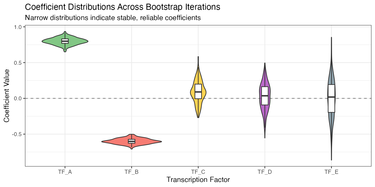
Step 4: Bootstrap Aggregation

Algorithm

# Pseudocode for bagging
bagging_coefficients <- function(X, y, n_bootstrap = 200, sample_ratio = 0.8) {
  n_cells <- ncol(X)
  n_sample <- floor(n_cells * sample_ratio)
  
  coef_list <- list()
  
  for (b in 1:n_bootstrap) {
    # Random subsample without replacement
    idx <- sample(n_cells, n_sample, replace = FALSE)
    
    # Fit Ridge regression
    coef_list[[b]] <- ridge_fit(X[, idx], y[idx], alpha = 10)
  }
  
  # Aggregate: use median (robust to outliers)
  final_coef <- apply(do.call(cbind, coef_list), 1, median)
  
  return(final_coef)
}

Coefficient Stability Assessment

Step 5: Links Object

The Links class stores and analyzes the fitted GRN:

# Get Links object from Oracle
links <- oracle$get_links(
  cluster_name_for_GRN_unit = "Cluster1"
)

# Explore the network
links$filter(
  threshold_p = 0.001,      # p-value threshold
  threshold_coef = 0.1      # coefficient magnitude threshold
)

# Calculate network metrics
links$get_network_score()

# Export for visualization
links$get_igraph()

Links Data Structure

Example Links Data Frame Structure
Source (TF)	Target (Gene)	Coefficient
TF_A	Gene_1	0.85
TF_A	Gene_2	0.42
TF_B	Gene_1	-0.61
TF_B	Gene_3	0.33
TF_C	Gene_2	0.71

Performance Considerations

Computational Complexity

Component	Time Complexity	Memory
Ridge regression	O(p³) per gene	O(p²)
Bagging (B iterations)	O(B × n × p³)	O(p²)
Full GRN	O(G × B × n × p³)	O(G × p)

Where: G = genes, n = cells, p = max TFs per gene, B = bootstrap iterations

Parallelization

CellOracleR uses the future package for parallel processing:

library(future)

# Setup parallel processing
plan(multisession, workers = 4)

# Now GRN fitting will use 4 cores
oracle$fit_grn_for_simulation(
  bagging_number = 200
)

# Reset to sequential
plan(sequential)

C++ Acceleration

Performance-critical operations are implemented in C++ via Rcpp:

Matrix multiplication in signal propagation
K-nearest neighbor weight calculation
Correlation computation
Markov chain simulation

Best Practices

1. Data Quality

# Filter before GRN inference
seurat_obj <- subset(seurat_obj, 
                     nFeature_RNA > 500 & 
                     nCount_RNA > 1000 &
                     percent.mt < 20)

2. Appropriate Clustering

Use biological meaningful clusters
Aim for 500-5000 cells per cluster
Very small clusters may produce unstable GRNs

3. TF-Target Prior Quality

High-quality priors improve inference accuracy
Consider using multiple evidence sources
Validate key relationships when possible

Summary

The CellOracleR GRN inference pipeline:

Prepares expression data and TF-target priors
Fits cluster-specific Ridge regression models
Stabilizes estimates through bootstrap aggregation
Stores results in the Links class for downstream analysis

This produces robust, interpretable gene regulatory networks suitable for perturbation simulation.

Session Info

sessionInfo()
#> R version 4.4.0 (2024-04-24)
#> Platform: aarch64-apple-darwin20
#> Running under: macOS 15.6.1
#> 
#> Matrix products: default
#> BLAS:   /Library/Frameworks/R.framework/Versions/4.4-arm64/Resources/lib/libRblas.0.dylib 
#> LAPACK: /Library/Frameworks/R.framework/Versions/4.4-arm64/Resources/lib/libRlapack.dylib;  LAPACK version 3.12.0
#> 
#> locale:
#> [1] C
#> 
#> time zone: Asia/Shanghai
#> tzcode source: internal
#> 
#> attached base packages:
#> [1] stats     graphics  grDevices utils     datasets  methods   base     
#> 
#> other attached packages:
#> [1] Matrix_1.7-4  ggplot2_4.0.1
#> 
#> loaded via a namespace (and not attached):
#>  [1] gtable_0.3.6       jsonlite_2.0.0     dplyr_1.1.4        compiler_4.4.0    
#>  [5] tidyselect_1.2.1   dichromat_2.0-0.1  jquerylib_0.1.4    splines_4.4.0     
#>  [9] systemfonts_1.3.1  scales_1.4.0       textshaping_1.0.4  yaml_2.3.12       
#> [13] fastmap_1.2.0      lattice_0.22-7     R6_2.6.1           labeling_0.4.3    
#> [17] generics_0.1.4     knitr_1.51         htmlwidgets_1.6.4  tibble_3.3.1      
#> [21] desc_1.4.3         bslib_0.9.0        pillar_1.11.1      RColorBrewer_1.1-3
#> [25] rlang_1.1.7        cachem_1.1.0       xfun_0.56          fs_1.6.6          
#> [29] sass_0.4.10        S7_0.2.1           otel_0.2.0         cli_3.6.5         
#> [33] mgcv_1.9-3         pkgdown_2.1.3      withr_3.0.2        magrittr_2.0.4    
#> [37] digest_0.6.39      grid_4.4.0         nlme_3.1-168       lifecycle_1.0.5   
#> [41] vctrs_0.7.1        evaluate_1.0.5     glue_1.8.0         farver_2.1.2      
#> [45] ragg_1.5.0         rmarkdown_2.30     tools_4.4.0        pkgconfig_2.0.3   
#> [49] htmltools_0.5.9

Building Gene Regulatory Networks from Single-Cell Data

Zaoqu Liu

2026-01-25