Algorithm Principles

Introduction

CellOracleR implements a mathematical framework for predicting cell state transitions following transcription factor (TF) perturbations. This vignette describes the core algorithms underlying the package.

1. Gene Regulatory Network (GRN) Inference

1.1 Mathematical Formulation

For each target gene $g$ , we model its expression as a linear function of its regulators:

$X_g = \sum_{r \in R_g} \beta_{r,g} \cdot X_r + \epsilon_g$

where:

$X_g$ is the expression of target gene $g$
$R_g$ is the set of regulators for gene $g$
$\beta_{r,g}$ is the regulatory coefficient from regulator $r$ to target $g$
$\epsilon_g$ is the residual error

1.2 Ridge Regression

We use Ridge regression (L2 regularization) to estimate $\beta$ coefficients:

$\hat{\beta} = \arg\min_\beta \left\{ \|X_g - X_R \beta\|_2^2 + \alpha \|\beta\|_2^2 \right\}$

The closed-form solution is:

$\hat{\beta} = (X_R^T X_R + \alpha I)^{-1} X_R^T X_g$

Why Ridge Regression?

Prevents overfitting: Regularization shrinks coefficients toward zero
Handles multicollinearity: Correlated regulators don’t cause instability
Numerical stability: Always has a unique solution

# Ridge regression in CellOracleR
coef_matrix <- fit_grn_coef_matrix(
  gem = expression_matrix,
  TFdict = tf_target_dict,
  alpha = 10  # regularization strength
)

1.3 Bootstrap Aggregation (Bagging)

To improve robustness, we employ bagging:

Sample 80% of cells (without replacement)
Fit Ridge regression on the subsample
Repeat $B$ times (typically 200)
Use median of coefficients as final estimate

$\hat{\beta}_{final} = \text{median}(\hat{\beta}_1, \hat{\beta}_2, \ldots, \hat{\beta}_B)$

Advantages:

Reduces variance of coefficient estimates
More robust to outlier cells
Provides coefficient stability measures

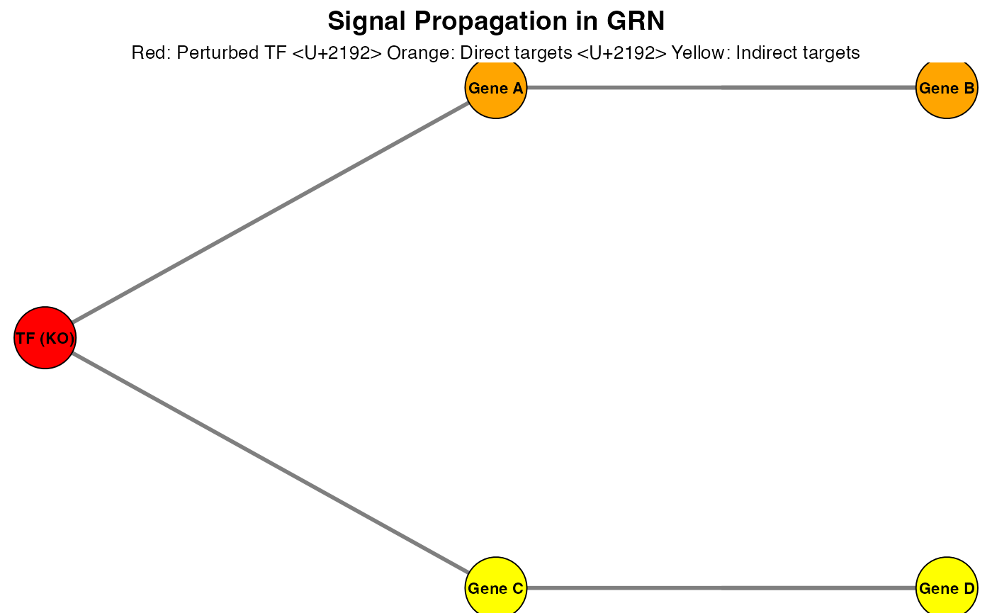
2. Signal Propagation Simulation

2.1 Perturbation Model

Given a perturbation condition (e.g., TF knockout), we simulate the downstream effects:

$\Delta X^{(0)} = X_{perturbed} - X_{original}$

2.2 Iterative Propagation

The signal propagates through the GRN iteratively:

$\Delta X^{(t+1)} = \Delta X^{(t)} \cdot W$

where $W$ is the coefficient matrix (genes × genes).

Key constraint: Perturbed gene values are maintained at each step:

$\Delta X^{(t+1)}_p = \Delta X^{(0)}_p \quad \text{for all perturbed genes } p$

2.3 Non-negativity Constraint

Gene expression cannot be negative:

$X_{simulated} = \max(0, X_{original} + \Delta X)$

Signal propagation through GRN

3. Transition Probability Estimation

3.1 Correlation-Based Approach

We estimate the probability of cell $i$ transitioning to cell $j$ based on:

$\rho_{ij} = \text{cor}(\Delta X_i, X_j - X_i)$

This measures how well the predicted expression change aligns with the direction toward cell $j$ .

3.2 Probability Conversion

Correlations are converted to probabilities using an exponential kernel:

$P_{ij} = \frac{\exp(\rho_{ij} / \sigma)}{\sum_{k \in N_i} \exp(\rho_{ik} / \sigma)}$

where:

$N_i$ is the set of k-nearest neighbors of cell $i$
$\sigma$ is a bandwidth parameter (default: 0.05)

3.3 Embedding Shift Calculation

The expected movement in embedding space:

$\Delta E_i = \sum_{j \in N_i} P_{ij} \cdot \hat{d}_{ij}$

where $\hat{d}_{ij}$ is the unit vector from cell $i$ to cell $j$ in embedding space.

4. Markov Chain Simulation

4.1 State Transition Model

Cell fate is modeled as a discrete-time Markov chain:

$P(S_{t+1} = j | S_t = i) = P_{ij}$

4.2 Trajectory Simulation

For each starting cell, we simulate $N$ steps:

Algorithm: Markov Walk
Input: transition_prob P, start_cell s, n_steps T
Output: trajectory [s_0, s_1, ..., s_T]

s_0 ← s
for t = 1 to T:
    sample s_t from Categorical(P[s_{t-1}, :])
return [s_0, s_1, ..., s_T]

4.3 Fate Probability

For absorbing Markov chains, we can compute the probability of reaching each terminal state:

$F = (I - Q)^{-1} R$

where $Q$ is the transient-to-transient transition matrix and $R$ is the transient-to-absorbing matrix.

5. Network Analysis Metrics

5.1 Centrality Measures

Degree centrality: $C_D(v) = \text{deg}(v) = |N(v)|$

Betweenness centrality: $C_B(v) = \sum_{s \neq v \neq t} \frac{\sigma_{st}(v)}{\sigma_{st}}$

Eigenvector centrality: $C_E(v) = \frac{1}{\lambda} \sum_{u \in N(v)} C_E(u)$

5.2 Network Entropy

Degree distribution entropy:

$H = -\sum_{k} p(k) \log_2 p(k)$

Higher entropy indicates more heterogeneous connectivity.

Summary

CellOracleR combines:

Ridge regression for robust GRN inference
Signal propagation for perturbation simulation
Correlation-based transition probabilities for fate prediction
Markov chains for trajectory modeling
Graph theory for network analysis

These mathematical foundations enable accurate prediction of cellular responses to genetic perturbations.

References

Kamimoto, K., et al. (2023). CellOracle: Dissecting cell identity via network inference and in silico gene perturbation. Molecular Systems Biology.
Hoerl, A.E. & Kennard, R.W. (1970). Ridge Regression: Biased Estimation for Nonorthogonal Problems. Technometrics.
Breiman, L. (1996). Bagging Predictors. Machine Learning.

Session Info

sessionInfo()
#> R version 4.4.0 (2024-04-24)
#> Platform: aarch64-apple-darwin20
#> Running under: macOS 15.6.1
#> 
#> Matrix products: default
#> BLAS:   /Library/Frameworks/R.framework/Versions/4.4-arm64/Resources/lib/libRblas.0.dylib 
#> LAPACK: /Library/Frameworks/R.framework/Versions/4.4-arm64/Resources/lib/libRlapack.dylib;  LAPACK version 3.12.0
#> 
#> locale:
#> [1] C
#> 
#> time zone: Asia/Shanghai
#> tzcode source: internal
#> 
#> attached base packages:
#> [1] stats     graphics  grDevices utils     datasets  methods   base     
#> 
#> other attached packages:
#> [1] ggplot2_4.0.1
#> 
#> loaded via a namespace (and not attached):
#>  [1] gtable_0.3.6       jsonlite_2.0.0     dplyr_1.1.4        compiler_4.4.0    
#>  [5] tidyselect_1.2.1   dichromat_2.0-0.1  jquerylib_0.1.4    systemfonts_1.3.1 
#>  [9] scales_1.4.0       textshaping_1.0.4  yaml_2.3.12        fastmap_1.2.0     
#> [13] R6_2.6.1           labeling_0.4.3     generics_0.1.4     knitr_1.51        
#> [17] htmlwidgets_1.6.4  tibble_3.3.1       desc_1.4.3         bslib_0.9.0       
#> [21] pillar_1.11.1      RColorBrewer_1.1-3 rlang_1.1.7        cachem_1.1.0      
#> [25] xfun_0.56          fs_1.6.6           sass_0.4.10        S7_0.2.1          
#> [29] otel_0.2.0         cli_3.6.5          pkgdown_2.1.3      withr_3.0.2       
#> [33] magrittr_2.0.4     digest_0.6.39      grid_4.4.0         lifecycle_1.0.5   
#> [37] vctrs_0.7.1        evaluate_1.0.5     glue_1.8.0         farver_2.1.2      
#> [41] ragg_1.5.0         rmarkdown_2.30     tools_4.4.0        pkgconfig_2.0.3   
#> [45] htmltools_0.5.9

Mathematical Foundations of CellOracleR

Zaoqu Liu

2026-01-25