Getting Started with CellOracleR

Introduction

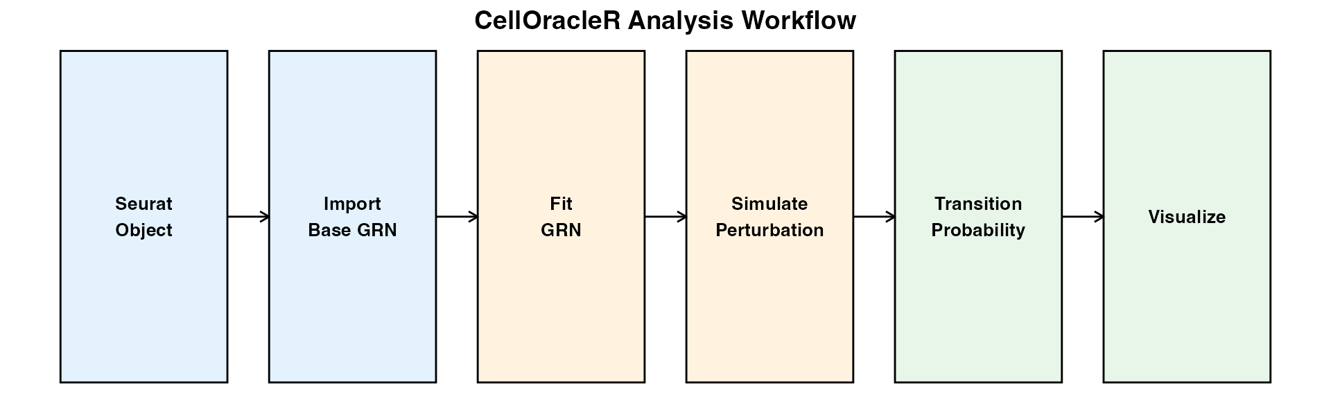
CellOracleR enables in silico gene perturbation analysis of single-cell RNA-seq data. By combining gene regulatory network (GRN) inference with expression data, CellOracleR predicts cell state transitions in response to transcription factor perturbations.

Key Features

R6 Object-Oriented Design: Clean, intuitive API
Seurat Integration: Seamless workflow with Seurat V4/V5
High Performance: C++ acceleration for critical operations
Publication-Ready Visualizations: ggplot2-based plotting functions
Comprehensive Network Analysis: Centrality metrics, hub detection, and more

Workflow Overview

Installation

# Install from R-universe (recommended)
install.packages("CellOracleR", repos = "https://zaoqu-liu.r-universe.dev")

# Or install from GitHub
devtools::install_github("Zaoqu-Liu/CellOracleR")

# For motif analysis, install Bioconductor dependencies
BiocManager::install(c(
  "TFBSTools", "motifmatchr", 
  "BSgenome.Hsapiens.UCSC.hg38", "JASPAR2020"
))

Load Libraries

library(CellOracleR)
library(Seurat)
library(ggplot2)
library(future)

# Enable parallel processing (optional)
plan(multisession, workers = 4)

Step 1: Prepare Data

CellOracleR works with standard Seurat objects. The data should be normalized (log-transformed) but NOT scaled/centered.

# Load your Seurat object
seurat <- readRDS("path/to/seurat.rds")

# Check data structure
seurat

Creating Demo Data

For this tutorial, we’ll create a mock dataset:

set.seed(42)
n_cells <- 1000
n_genes <- 500

# Simulate expression with cluster structure
cluster_means <- list(
  c1 = c(rep(3, 50), rep(1, 450)),  # Cluster 1: high expression in first 50 genes
  c2 = c(rep(1, 50), rep(3, 100), rep(1, 350)),  # Cluster 2
  c3 = c(rep(1, 150), rep(3, 100), rep(1, 250))  # Cluster 3
)

# Create expression matrix
cells_per_cluster <- 333
expr_list <- list()
for (i in 1:3) {
  expr_list[[i]] <- matrix(
    rpois(cells_per_cluster * n_genes, lambda = cluster_means[[i]]),
    nrow = n_genes
  )
}
counts <- do.call(cbind, expr_list)
rownames(counts) <- paste0("Gene", 1:n_genes)
colnames(counts) <- paste0("Cell", 1:ncol(counts))

# Create Seurat object
seurat <- CreateSeuratObject(counts = counts)
seurat <- NormalizeData(seurat)
seurat <- FindVariableFeatures(seurat)
seurat <- ScaleData(seurat)
seurat <- RunPCA(seurat)
seurat <- FindNeighbors(seurat, dims = 1:30)
seurat <- FindClusters(seurat, resolution = 0.5)
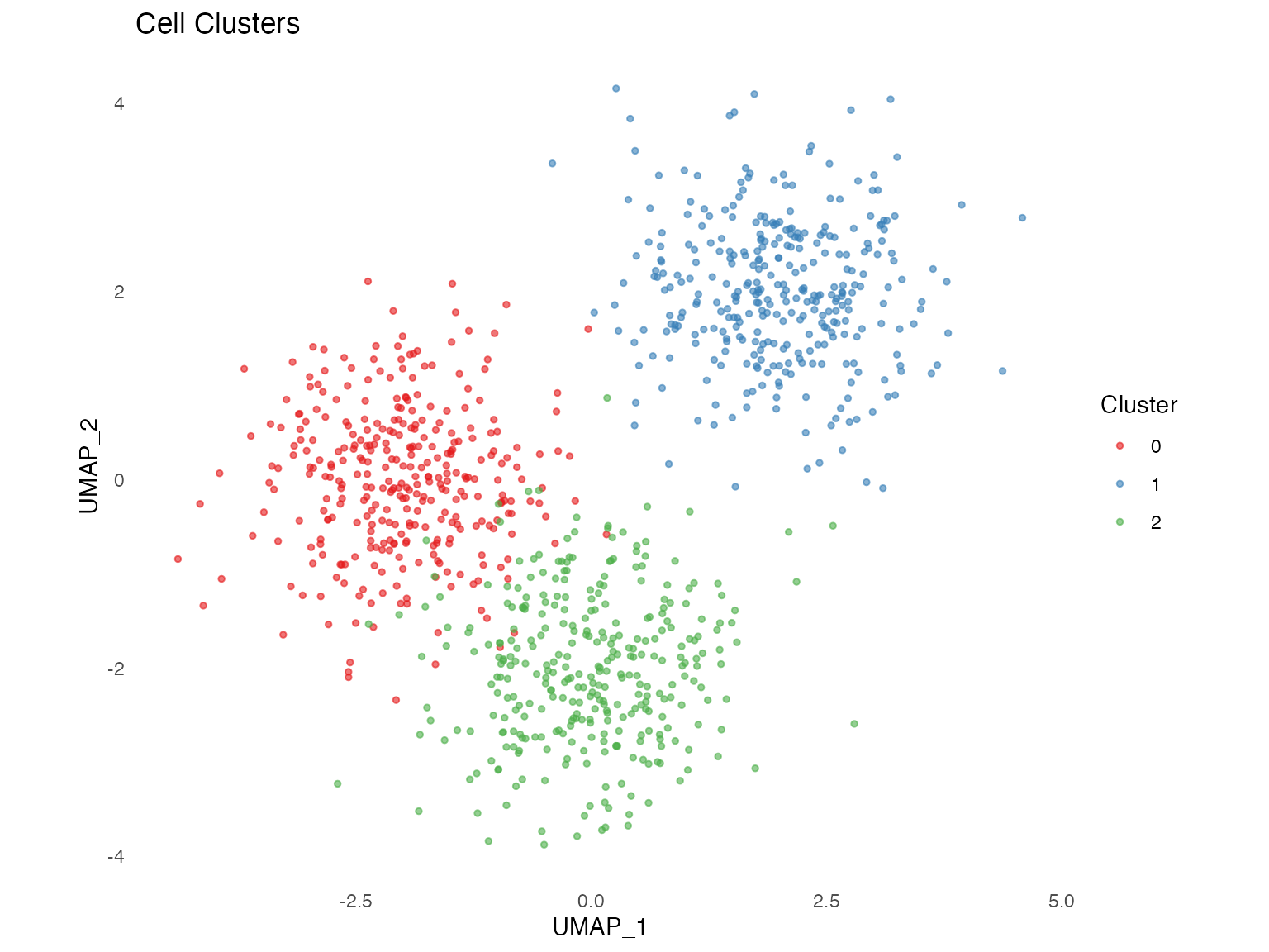
seurat <- RunUMAP(seurat, dims = 1:30)

Step 2: Create Oracle Object

# Create Oracle from Seurat
oracle <- create_oracle(
  seurat = seurat,
  cluster_column = "seurat_clusters",
  embedding_name = "umap",
  verbose = TRUE
)

# Print summary
oracle

Output:

CellOracleR Oracle Object
  Cells: 1000
  Genes: 500
  Clusters: 3 (0, 1, 2)
  Embedding: UMAP (2D)
  GRN fitted: FALSE
  Simulation done: FALSE

Step 3: Import Base GRN

The base GRN defines which TFs can potentially regulate which genes. Options:

Option A: From Motif Analysis (Recommended)

# Requires scATAC-seq peak data
base_grn <- create_base_grn(
  peaks_df = peaks_df,        # data.frame with chr, start, end, gene_short_name
  ref_genome = "hg38",
  upstream = 2000,
  downstream = 2000,
  fpr = 0.02,
  n_cores = 4
)

Option B: From Pre-built Database

# Load from CSV file
base_grn <- load_base_grn("tf_target_database.csv")

Option C: Custom Dictionary

# Define regulatory relationships manually
# List format: target_gene -> c(regulator1, regulator2, ...)
TFdict <- list(
  Gene1 = c("Gene10", "Gene20", "Gene30"),
  Gene2 = c("Gene10", "Gene15", "Gene25"),
  Gene3 = c("Gene20", "Gene30", "Gene40")
)

# For demo: create simple TF dictionary
TFdict <- lapply(paste0("Gene", 1:100), function(g) {
  sample(paste0("Gene", 101:200), size = sample(3:8, 1))
})
names(TFdict) <- paste0("Gene", 1:100)

Import to Oracle

oracle$import_TF_data(TFdict = TFdict)

Step 4: Preprocessing

# Use Seurat's PCA or compute new
oracle$perform_PCA(
  n_components = 50,
  use_seurat_pca = TRUE  # Use existing PCA from Seurat
)

# KNN imputation for noise reduction (optional but recommended)
oracle$knn_imputation(
  k = 30,           # Number of neighbors (NULL for auto)
  n_pca_dims = 50   # PCA dimensions for neighbor search
)

Step 5: Fit Cluster-Specific GRN

This is the core step - fitting regulatory coefficients using Ridge regression:

oracle$fit_grn_for_simulation(
  GRN_unit = "cluster",     # Fit separate GRN per cluster
  alpha = 10,               # Ridge regularization (1-100)
  bagging_number = 200,     # Bootstrap iterations
  verbose = TRUE
)

Key Parameters:

Parameter	Description	Recommended
`GRN_unit`	“cluster” or “whole”	“cluster”
`alpha`	Regularization strength	10
`bagging_number`	Bootstrap iterations	200

Step 6: Simulate Perturbation

Now we can simulate the effects of gene perturbations:

# Define perturbation: Gene10 knockout (expression = 0)
perturb_condition <- list(Gene10 = 0)

# Or use helper function
perturb_condition <- create_perturb_condition(
  genes = "Gene10",
  expression = 0
)

# Run simulation
oracle$simulate_shift(
  perturb_condition = perturb_condition,
  n_propagation = 3  # Signal propagation steps (1-5)
)

# View summary
simulation_summary(oracle)

Perturbation Types:

# Knockout (KO): Set expression to 0
perturb_ko <- list(Gene10 = 0)

# Overexpression (OE): Set to maximum observed value
max_expr <- max(oracle$adata$layers$imputed_count["Gene10", ])
perturb_oe <- list(Gene10 = max_expr)

# Multiple perturbations
perturb_multi <- list(
  Gene10 = 0,      # KO Gene10
  Gene20 = max_expr # OE Gene20
)

Step 7: Calculate Transition Probabilities

# Compute transition probabilities
oracle$estimate_transition_prob(
  k = 200,                   # KNN neighbors
  sampled_fraction = 1,      # Cell sampling fraction
  calculate_randomized = TRUE
)

# Calculate embedding shifts
oracle$calculate_embedding_shift()

# Calculate grid arrows for visualization
oracle$calculate_grid_arrows(
  n_grid = 40,
  n_neighbors = 100,
  smooth = 0.5
)

Step 8: Visualize Results

Cluster Overview

# Plot clusters
plot_cluster(oracle, title = "Cell Clusters")

Simulation Flow Field

The main visualization showing predicted cell state transitions:

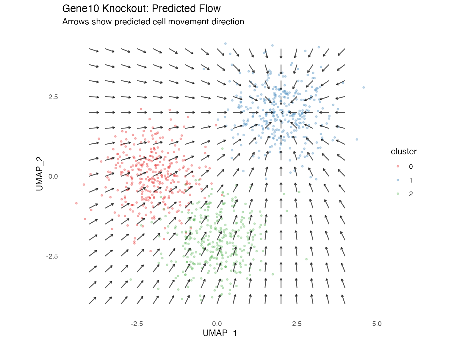
# Main result visualization
plot_simulation_flow(
  oracle,
  scale = 30,
  min_mass = 0.01,
  arrow_color = "black",
  title = "Gene10 KO: Predicted Cell Transitions"
)

Gene Expression Changes

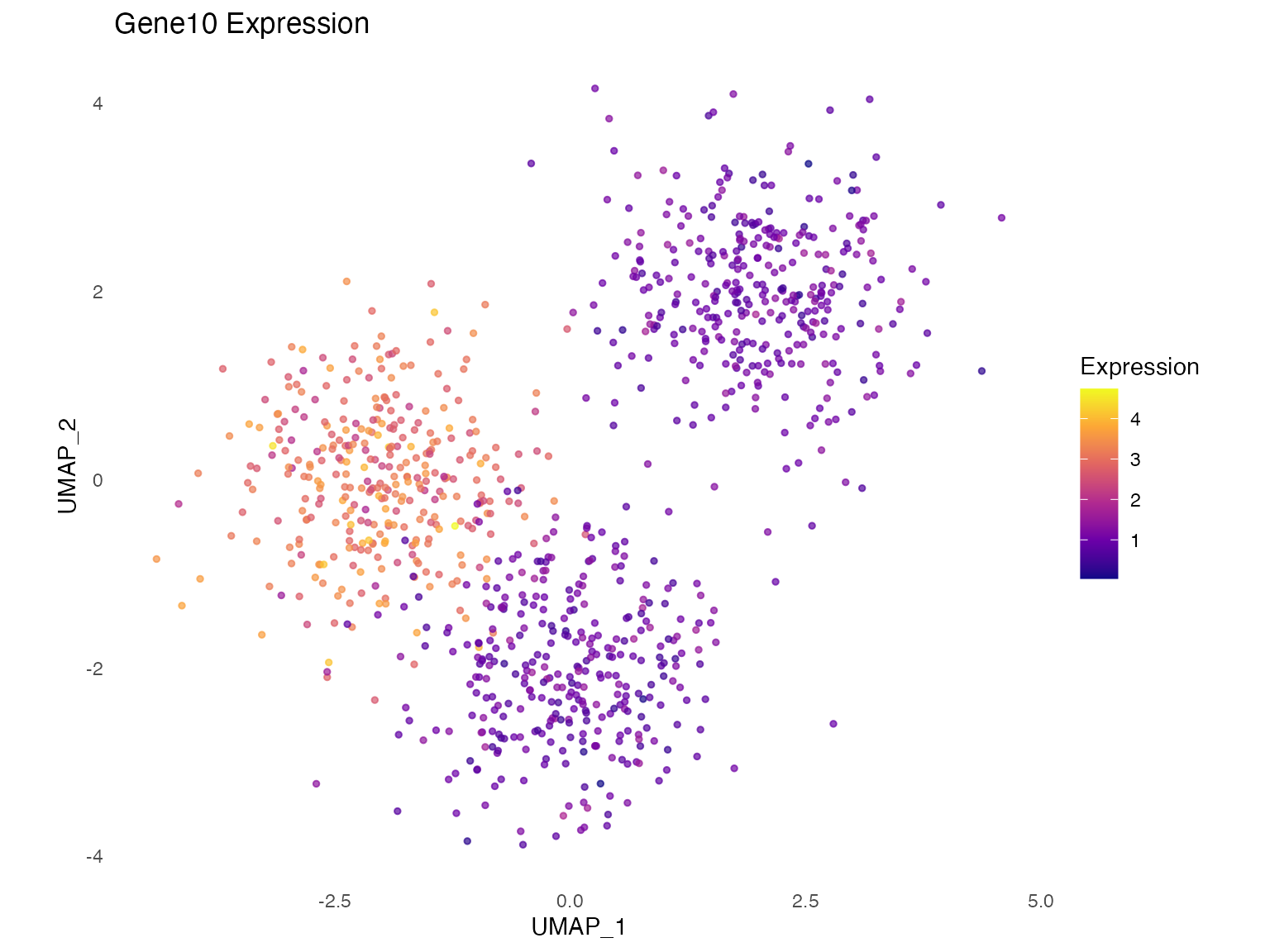
# Before perturbation
plot_gene_expression(oracle, "Gene10", title = "Gene10 Expression")

# Simulated change
plot_gene_expression(oracle, "Gene10", layer = "delta_X", 
                     title = "Gene10 Change (Delta)")

Step 9: Network Analysis

For detailed network characterization:

# Get Links object
links <- oracle$get_links(
  cluster_name_for_GRN_unit = "0",  # Cluster name
  alpha = 10,
  bagging_number = 200
)

# Filter by significance
links$filter(
  threshold_p = 0.001,
  threshold_coef = 0.1
)

# Calculate network metrics
links$get_network_score()

# View network summary
print(links)

Top Regulators

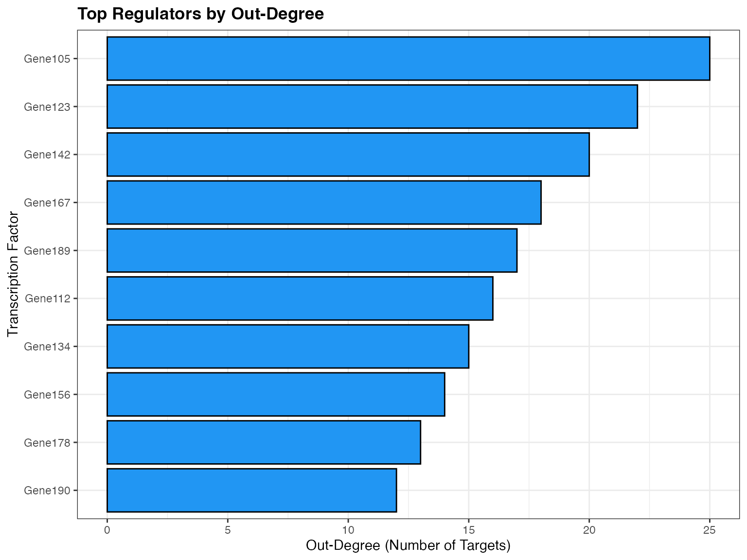
# Rank TFs by network metrics
plot_scores_as_rank(links, metric = "degree_out", top_n = 20)

Saving and Loading

# Save Oracle object (uses qs for fast serialization)
save_oracle(oracle, "my_analysis.qs")

# Load Oracle object
oracle <- load_oracle("my_analysis.qs")

Advanced: Comparing Multiple Perturbations

# List of genes to perturb
genes_to_test <- c("Gene10", "Gene20", "Gene30")

# Run systematic analysis
plots <- list()
for (gene in genes_to_test) {
  # Create copy to avoid overwriting
  oracle_test <- oracle$clone(deep = TRUE)
  
  # Simulate knockout
  oracle_test$simulate_shift(
    perturb_condition = list(gene = 0),
    n_propagation = 3
  )
  
  # Calculate transitions
  oracle_test$estimate_transition_prob()
  oracle_test$calculate_embedding_shift()
  oracle_test$calculate_grid_arrows()
  
  # Store plot
  plots[[gene]] <- plot_simulation_flow(oracle_test, title = paste(gene, "KO"))
}

# Combine plots
library(patchwork)
wrap_plots(plots, ncol = 2)

Summary

You’ve learned how to:

✅ Create an Oracle object from Seurat data
✅ Import regulatory network priors
✅ Fit cluster-specific GRNs
✅ Simulate gene perturbations
✅ Calculate transition probabilities
✅ Visualize predicted cell fate changes
✅ Perform network analysis

Next Steps

Read the Algorithm Principles vignette for mathematical details
Explore the Visualization Gallery for more plot types
See the Case Study for a complete biological example

Session Info

sessionInfo()
#> R version 4.4.0 (2024-04-24)
#> Platform: aarch64-apple-darwin20
#> Running under: macOS 15.6.1
#> 
#> Matrix products: default
#> BLAS:   /Library/Frameworks/R.framework/Versions/4.4-arm64/Resources/lib/libRblas.0.dylib 
#> LAPACK: /Library/Frameworks/R.framework/Versions/4.4-arm64/Resources/lib/libRlapack.dylib;  LAPACK version 3.12.0
#> 
#> locale:
#> [1] C
#> 
#> time zone: Asia/Shanghai
#> tzcode source: internal
#> 
#> attached base packages:
#> [1] stats     graphics  grDevices utils     datasets  methods   base     
#> 
#> other attached packages:
#> [1] ggplot2_4.0.1
#> 
#> loaded via a namespace (and not attached):
#>  [1] gtable_0.3.6       jsonlite_2.0.0     dplyr_1.1.4        compiler_4.4.0    
#>  [5] tidyselect_1.2.1   dichromat_2.0-0.1  jquerylib_0.1.4    systemfonts_1.3.1 
#>  [9] scales_1.4.0       textshaping_1.0.4  yaml_2.3.12        fastmap_1.2.0     
#> [13] R6_2.6.1           labeling_0.4.3     generics_0.1.4     knitr_1.51        
#> [17] htmlwidgets_1.6.4  tibble_3.3.1       desc_1.4.3         bslib_0.9.0       
#> [21] pillar_1.11.1      RColorBrewer_1.1-3 rlang_1.1.7        cachem_1.1.0      
#> [25] xfun_0.56          fs_1.6.6           sass_0.4.10        S7_0.2.1          
#> [29] otel_0.2.0         viridisLite_0.4.2  cli_3.6.5          pkgdown_2.1.3     
#> [33] withr_3.0.2        magrittr_2.0.4     digest_0.6.39      grid_4.4.0        
#> [37] lifecycle_1.0.5    vctrs_0.7.1        evaluate_1.0.5     glue_1.8.0        
#> [41] farver_2.1.2       ragg_1.5.0         rmarkdown_2.30     tools_4.4.0       
#> [45] pkgconfig_2.0.3    htmltools_0.5.9

Complete Workflow for In Silico Gene Perturbation Analysis

Zaoqu Liu

2026-01-25