Mathematical Framework and Algorithm

Zaoqu Liu

2026-01-26

Introduction

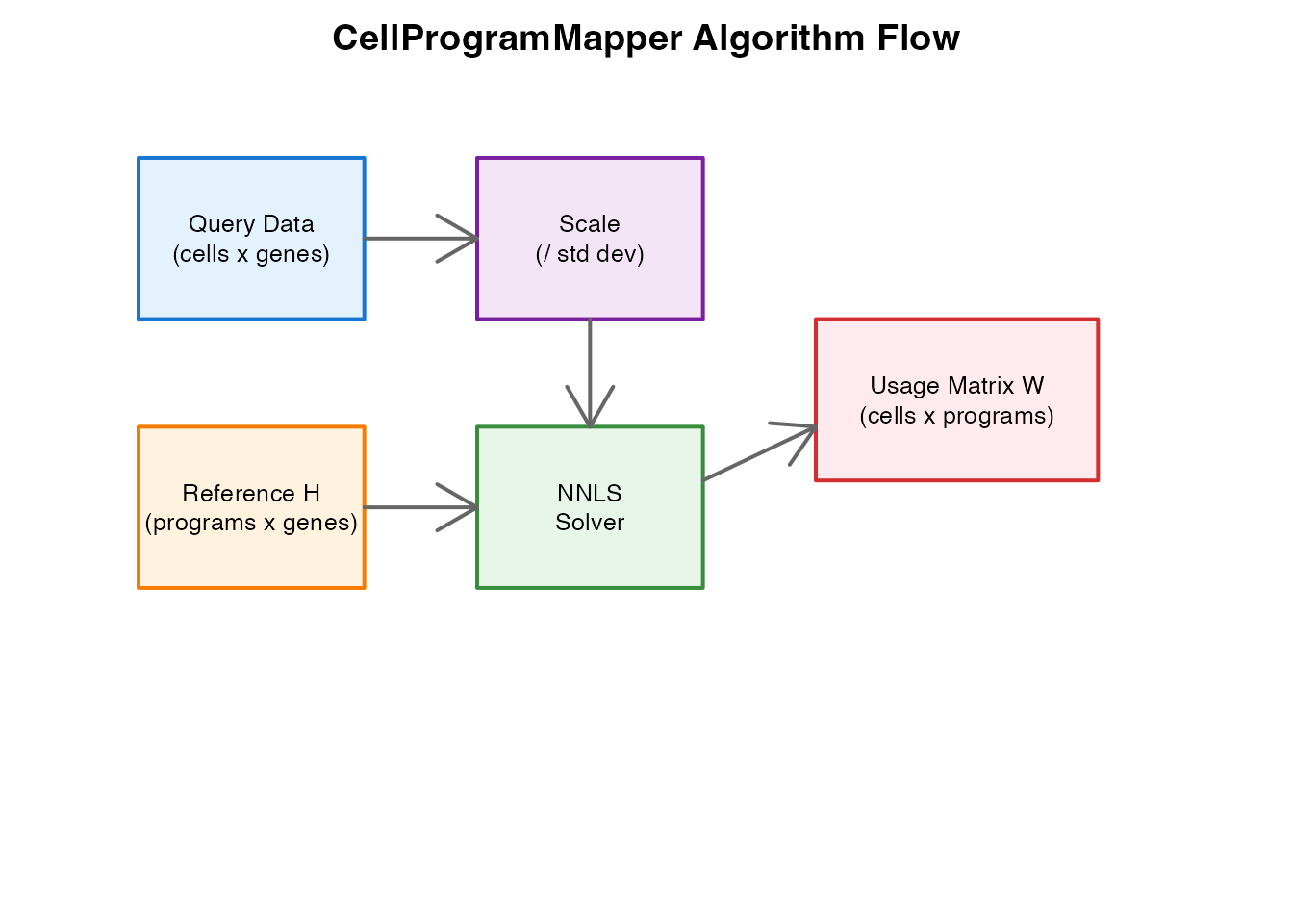
CellProgramMapper implements a projection-based approach for mapping single-cell transcriptomic data onto reference gene expression programs (GEPs). This vignette provides a detailed explanation of the mathematical framework underlying the algorithm.

Problem Formulation

Non-Negative Matrix Factorization (NMF)

Gene expression programs are typically discovered using Non-Negative Matrix Factorization (NMF). Given an expression matrix $\mathbf{X} \in \mathbb{R}^{n \times p}$ (n cells x p genes), NMF seeks to find:

$$\mathbf{X} \approx \mathbf{W} \mathbf{H}$$

where:

• $\mathbf{W} \in \mathbb{R}^{n \times k}$: Usage matrix (n cells x k programs)
• $\mathbf{H} \in \mathbb{R}^{k \times p}$: Spectra matrix (k programs x p genes)

The non-negativity constraints $\mathbf{W} \geq 0$ and $\mathbf{H} \geq 0$ ensure biological interpretability.

Projection Problem

CellProgramMapper addresses a related but distinct problem: given a fixed reference spectra matrix $\mathbf{H}$, estimate the usage matrix $\mathbf{W}$ for new query data $\mathbf{X}$.

This is formulated as:

$$\min_{\mathbf{W} \geq 0} \|\mathbf{X} - \mathbf{W}\mathbf{H}\|_F^2$$

where $\|\cdot\|_F$ denotes the Frobenius norm.

Cell-wise Decomposition

The objective function decomposes over cells:

$$\|\mathbf{X} - \mathbf{W}\mathbf{H}\|_F^2 = \sum_{i=1}^{n} \|\mathbf{x}_i - \mathbf{H}^\top \mathbf{w}_i\|_2^2$$

where $\mathbf{x}_i \in \mathbb{R}^{p}$ is the expression vector for cell $i$, and $\mathbf{w}_i \in \mathbb{R}^{k}$ is its usage vector.

This allows us to solve $n$ independent Non-Negative Least Squares (NNLS) problems:

$$\min_{\mathbf{w}_i \geq 0} \|\mathbf{x}_i - \mathbf{H}^\top \mathbf{w}_i\|_2^2$$

NNLS Problem

Standard Form

The general NNLS problem is:

$$\min_{\mathbf{x} \geq 0} \|\mathbf{A}\mathbf{x} - \mathbf{b}\|_2^2$$

In our context:

• $\mathbf{A} = \mathbf{H}^\top$ (p genes x k programs)
• $\mathbf{x} = \mathbf{w}_i$ (k programs x 1)
• $\mathbf{b} = \mathbf{x}_i$ (p genes x 1)

KKT Conditions

The optimal solution satisfies the Karush-Kuhn-Tucker (KKT) conditions:

1. Primal feasibility: $\mathbf{x}^* \geq 0$
2. Stationarity: $\nabla f(\mathbf{x}^*) = \mathbf{A}^\top(\mathbf{A}\mathbf{x}^* - \mathbf{b}) \geq 0$ for components where $x_j^* = 0$
3. Complementary slackness: $x_j^* \cdot [\mathbf{A}^\top(\mathbf{A}\mathbf{x}^* - \mathbf{b})]_j = 0$

Data Preprocessing

Scaling

Before NNLS fitting, the query data is scaled by dividing each gene by its population standard deviation (without centering):

$$x'_{ij} = \frac{x_{ij}}{\sigma_j}$$

where:

$$\sigma_j = \sqrt{\frac{1}{n}\sum_{i=1}^n (x_{ij} - \bar{x}_j)^2}$$

This matches the preprocessing used in Python’s sklearn.preprocessing.scale(X, with_mean=False) and ensures consistency with the Python implementation.

Why Not Center?

Centering (subtracting the mean) is avoided because:

1. Single-cell count data is inherently non-negative
2. Centering would violate the non-negativity assumption
3. The reference spectra are trained on non-centered data

Usage Normalization

After obtaining the raw usage matrix $\mathbf{W}$, rows are normalized to sum to 1:

$$\tilde{w}_{ij} = \frac{w_{ij}}{\sum_{l=1}^{k} w_{il}}$$

This normalized usage represents the relative contribution of each program to a cell’s expression profile.

Computational Complexity

For a single cell with $p$ genes and $k$ programs:

• Active Set Method: $O(k^3)$ per iteration, $O(I \cdot k^3)$ total
• Coordinate Descent: $O(k^2)$ per iteration, $O(I \cdot k^2)$ total

where $I$ is the number of iterations.

For $n$ cells, the total complexity is $O(n \cdot I \cdot k^2)$ or $O(n \cdot I \cdot k^3)$.

Visualization of the Algorithm

Schematic of the CellProgramMapper algorithm

Example: Geometric Interpretation

The NNLS solution can be interpreted geometrically. Each cell’s expression profile is projected onto the non-negative cone spanned by the reference program spectra.

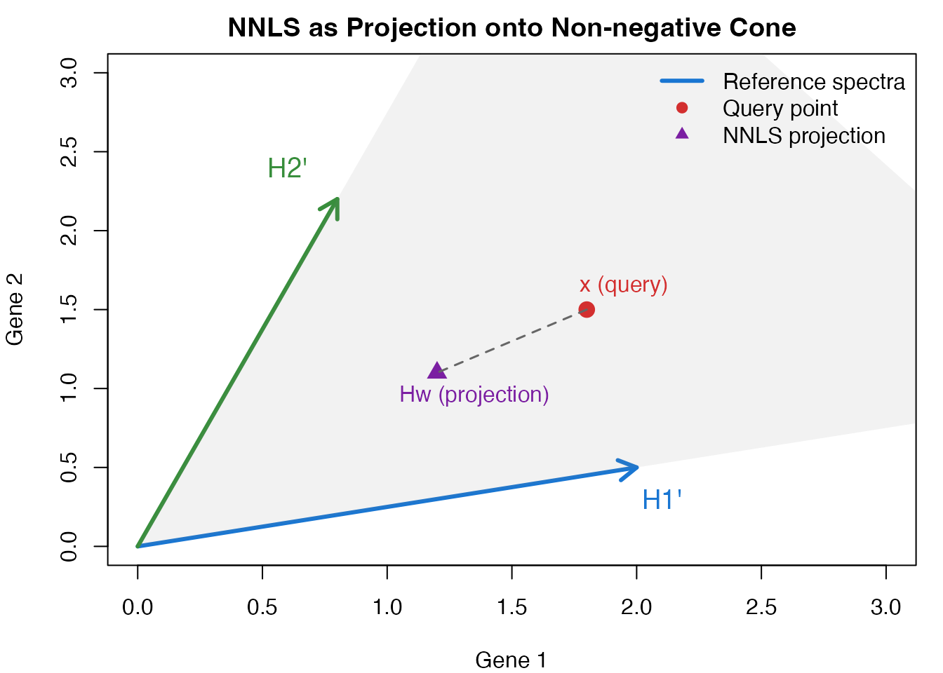
Geometric interpretation of NNLS projection

Summary

Component	Description
Input	Query matrix X (cells x genes), Reference H (programs x genes)
Output	Usage matrix W (cells x programs)
Preprocessing	Scale by population standard deviation
Solver	NNLS (Coordinate Descent or Active Set)
Post-processing	Row normalization (optional)

References

1. Lee DD, Seung HS (1999). Learning the parts of objects by non-negative matrix factorization. Nature 401:788-791.

2. Lawson CL, Hanson RJ (1974). Solving Least Squares Problems. Prentice-Hall.

3. Franc V, Hlavac V, Navara M (2005). Sequential Coordinate-Wise Algorithm for the Non-negative Least Squares Problem. CAIP 2005.

Session Info

sessionInfo()
#> R version 4.4.0 (2024-04-24)
#> Platform: aarch64-apple-darwin20
#> Running under: macOS 15.6.1
#> 
#> Matrix products: default
#> BLAS:   /Library/Frameworks/R.framework/Versions/4.4-arm64/Resources/lib/libRblas.0.dylib 
#> LAPACK: /Library/Frameworks/R.framework/Versions/4.4-arm64/Resources/lib/libRlapack.dylib;  LAPACK version 3.12.0
#> 
#> locale:
#> [1] C
#> 
#> time zone: Asia/Shanghai
#> tzcode source: internal
#> 
#> attached base packages:
#> [1] stats     graphics  grDevices utils     datasets  methods   base     
#> 
#> loaded via a namespace (and not attached):
#>  [1] digest_0.6.39     desc_1.4.3        R6_2.6.1          fastmap_1.2.0    
#>  [5] xfun_0.56         cachem_1.1.0      knitr_1.51        htmltools_0.5.9  
#>  [9] rmarkdown_2.30    lifecycle_1.0.5   cli_3.6.5         sass_0.4.10      
#> [13] pkgdown_2.2.0     textshaping_1.0.4 jquerylib_0.1.4   systemfonts_1.3.1
#> [17] compiler_4.4.0    tools_4.4.0       ragg_1.5.0        bslib_0.9.0      
#> [21] evaluate_1.0.5    yaml_2.3.12       otel_0.2.0        jsonlite_2.0.0   
#> [25] rlang_1.1.7       fs_1.6.6          htmlwidgets_1.6.4