Overview
This tutorial covers the communication analysis step, where production and sensing scores are combined to quantify cell-cell communication via metabolites.
library(scMetaLink)
library(Matrix)

# Load and prepare data
data(crc_example)
obj <- createScMetaLink(crc_expr, crc_meta, "cell_type")
obj <- inferProduction(obj, verbose = FALSE)
obj <- inferSensing(obj, verbose = FALSE)
Understanding Communication Scores
Communication from sender to receiver via metabolite:
Sender Cell ──[Production]──▶ Metabolite ──[Sensing]──▶ Receiver Cell
     │                            │                           │
     │                            │                           │
     ▼                            ▼                           ▼
  MPP(m,s)         ----->   Comm(s->r,m)   <-----         MSC(m,r)
The computeCommunication() Function
obj <- computeCommunication(
obj,
method = "geometric", # How to combine production and sensing
min_production = 0.1, # Minimum production threshold
min_sensing = 0.1, # Minimum sensing threshold
population.size = FALSE, # Weight by cell type abundance
n_permutations = 100, # Permutations for significance
n_cores = 1, # Parallel cores
seed = 42, # Reproducibility
verbose = TRUE
)
#> | | | 0% | |= | 1% | |= | 2% | |== | 3% | |=== | 4% | |==== | 5% | |==== | 6% | |===== | 7% | |====== | 8% | |====== | 9% | |======= | 10% | |======== | 11% | |======== | 12% | |========= | 13% | |========== | 14% | |========== | 15% | |=========== | 16% | |============ | 17% | |============= | 18% | |============= | 19% | |============== | 20% | |=============== | 21% | |=============== | 22% | |================ | 23% | |================= | 24% | |================== | 25% | |================== | 26% | |=================== | 27% | |==================== | 28% | |==================== | 29% | |===================== | 30% | |====================== | 31% | |====================== | 32% | |======================= | 33% | |======================== | 34% | |======================== | 35% | |========================= | 36% | |========================== | 37% | |=========================== | 38% | |=========================== | 39% | |============================ | 40% | |============================= | 41% | |============================= | 42% | |============================== | 43% | |=============================== | 44% | |================================ | 45% | |================================ | 46% | |================================= | 47% | |================================== | 48% | |================================== | 49% | |=================================== | 50% | |==================================== | 51% | |==================================== | 52% | |===================================== | 53% | |====================================== | 54% | |====================================== | 55% | |======================================= | 56% | |======================================== | 57% | |========================================= | 58% | |========================================= | 59% | |========================================== | 60% | |=========================================== | 61% | |=========================================== | 62% | |============================================ | 63% | |============================================= | 64% | |============================================== | 65% | |============================================== | 66% | |=============================================== | 67% | |================================================ | 68% | |================================================ | 69% | |================================================= | 70% | |================================================== | 71% | |================================================== | 72% | |=================================================== | 73% | |==================================================== | 74% | |==================================================== | 75% | |===================================================== | 76% | |====================================================== | 77% | |======================================================= | 78% | |======================================================= | 79% | |======================================================== | 80% | |========================================================= | 81% | |========================================================= | 82% | |========================================================== | 83% | |=========================================================== | 84% | |============================================================ | 85% | |============================================================ | 86% | |============================================================= | 87% | |============================================================== | 88% | |============================================================== | 89% | |=============================================================== | 90% | |================================================================ | 91% | |================================================================ | 92% | |================================================================= | 93% | |================================================================== | 94% | |================================================================== | 95% | |=================================================================== | 96% | |==================================================================== | 97% | |===================================================================== | 98% | |===================================================================== | 99% | |======================================================================| 100%Parameter Deep Dive
1. method: Combining Production and Sensing
Three methods to compute communication score:
# Run with different methods
obj_geom <- computeCommunication(obj, method = "geometric", n_permutations = 0, verbose = FALSE)
obj_prod <- computeCommunication(obj, method = "product", n_permutations = 0, verbose = FALSE)
obj_harm <- computeCommunication(obj, method = "harmonic", n_permutations = 0, verbose = FALSE)

# Compare total communication strength
par(mfrow = c(1, 3))

total_geom <- apply(obj_geom@communication_scores, c(1, 2), sum)
total_prod <- apply(obj_prod@communication_scores, c(1, 2), sum)
total_harm <- apply(obj_harm@communication_scores, c(1, 2), sum)

image(total_geom,
  main = "Geometric: sqrt(PxS)", col = hcl.colors(50, "YlOrRd"),
  axes = FALSE
)
image(total_prod,
  main = "Product: PxS", col = hcl.colors(50, "YlOrRd"),
  axes = FALSE
)
image(total_harm,
  main = "Harmonic: 2PS/(P+S)", col = hcl.colors(50, "YlOrRd"),
  axes = FALSE
)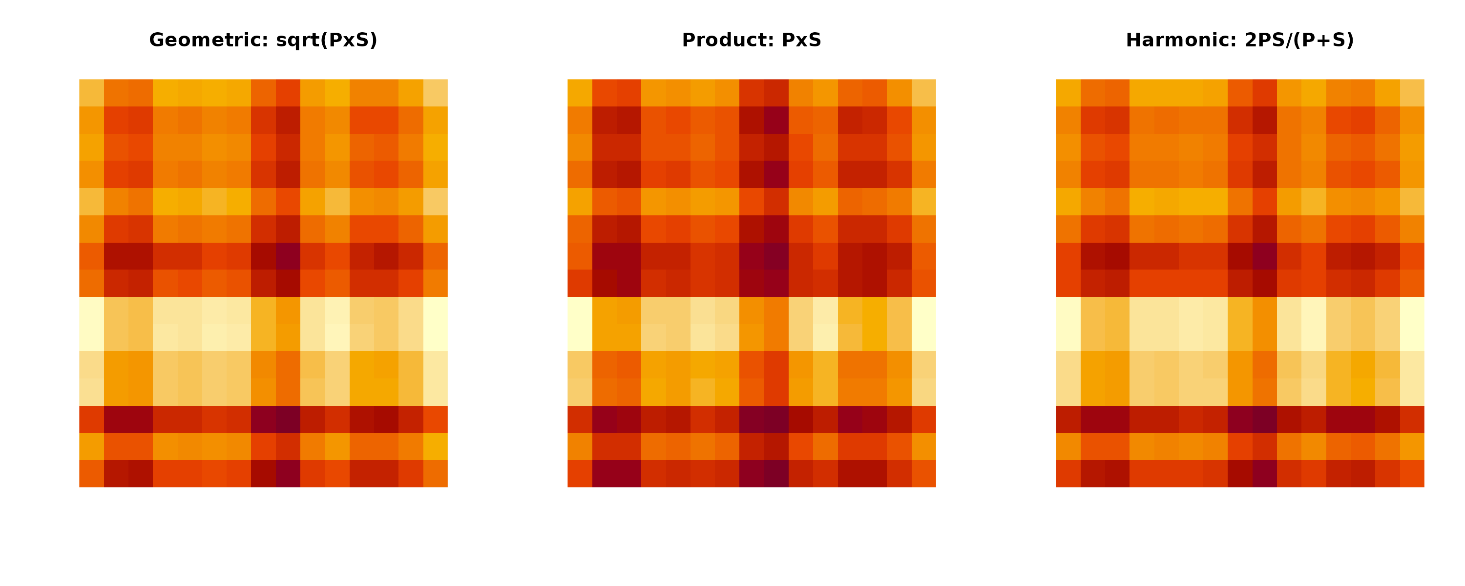
Figure 1: Communication Score Method Comparison. Heatmaps showing total communication strength between cell types using different aggregation methods. Geometric mean (default) provides balanced weighting, product emphasizes strong bilateral signals, and harmonic mean penalizes imbalanced communication.
Method recommendations:
| Method | Formula | Best for |
|---|---|---|
geometric |
General use, balanced | |
product |
Emphasizing strong bilateral signals | |
harmonic |
Penalizing imbalanced communication |
2. min_production and min_sensing: Noise
Filtering
# Compare different thresholds
thresholds <- c(0.05, 0.1, 0.2, 0.3)
n_interactions <- sapply(thresholds, function(t) {
  obj_t <- computeCommunication(obj,
    min_production = t, min_sensing = t,
    n_permutations = 0, verbose = FALSE
  )
  sum(obj_t@communication_scores > 0)
})

barplot(n_interactions,
  names.arg = thresholds,
  xlab = "Threshold (min_production = min_sensing)",
  ylab = "Number of Non-zero Interactions",
  main = "Effect of Thresholds on Detected Interactions",
  col = "#64B5F6"
)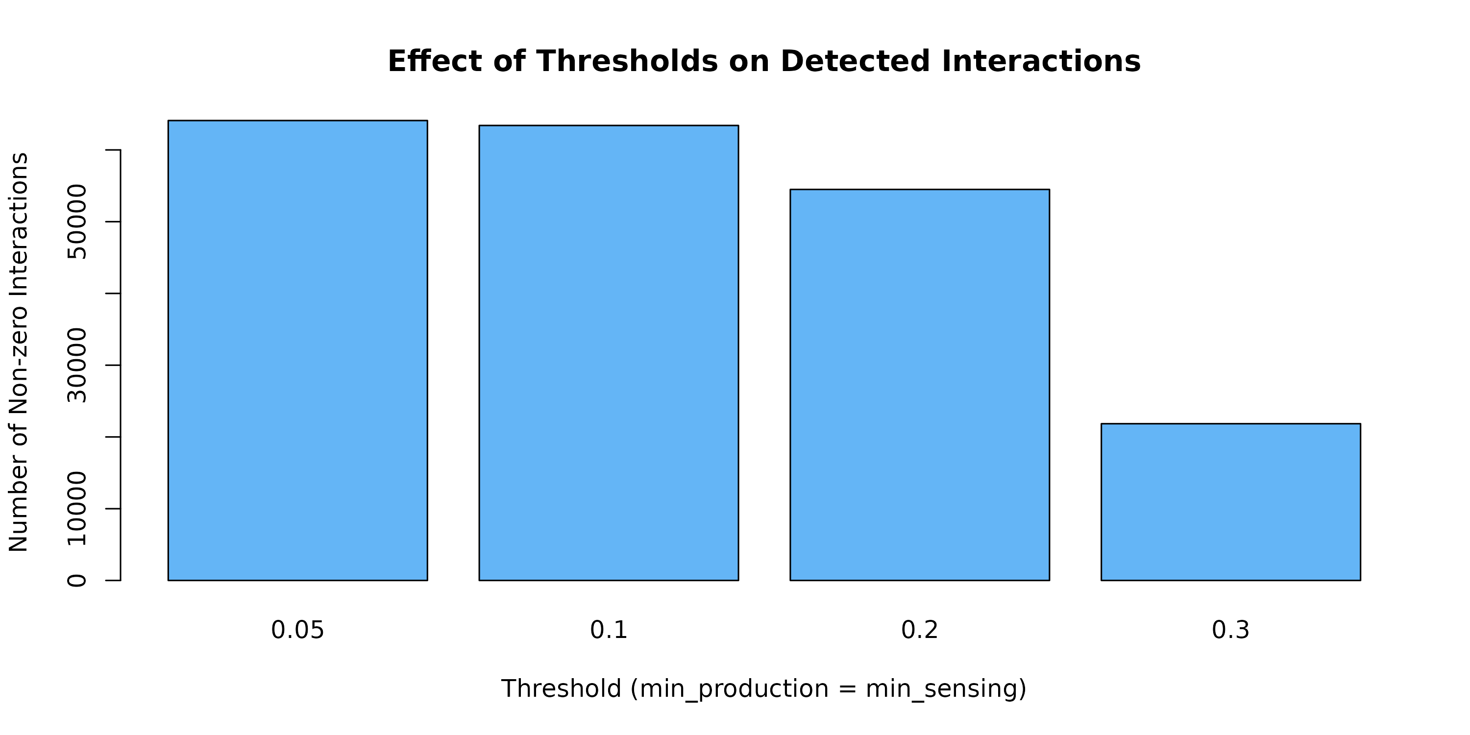
Figure 2: Effect of Expression Thresholds. Higher thresholds reduce the number of detected interactions by requiring stronger production and sensing signals. Choose based on desired stringency.
Guidelines: - 0.1: Default, moderate
filtering - 0.05: More permissive, may include noise -
0.2-0.3: More stringent, for focused analysis
3. population.size: Cell Type Abundance Weighting
When enabled, communication is weighted by cell type abundance:
# Compare with and without population size correction
obj_no_pop <- computeCommunication(obj,
  population.size = FALSE,
  n_permutations = 0, verbose = FALSE
)
obj_with_pop <- computeCommunication(obj,
  population.size = TRUE,
  n_permutations = 0, verbose = FALSE
)

# Total communication per cell type pair
total_no_pop <- apply(obj_no_pop@communication_scores, c(1, 2), sum)
total_with_pop <- apply(obj_with_pop@communication_scores, c(1, 2), sum)

cat("Without population size correction:\n")
#> Without population size correction:
print(round(total_no_pop[1:5, 1:5], 3))
#>                    receiver
#> sender              Normal Epithelial       T Plasma Normal Fibroblast     CAF
#>   Normal Epithelial            95.343 105.704 90.919           120.128 119.573
#>   T                            83.677  94.382 80.301           105.682 105.110
#>   Plasma                       83.028  93.692 80.557           104.482 103.873
#>   Normal Fibroblast            91.996 102.945 87.495           114.784 114.247
#>   CAF                          91.263 101.869 86.869           113.753 113.273

cat("\nWith population size correction:\n")
#>
#> With population size correction:
print(round(total_with_pop[1:5, 1:5], 3))
#>                    receiver
#> sender              Normal Epithelial      T Plasma Normal Fibroblast    CAF
#>   Normal Epithelial            10.036 14.365  8.737            10.325 10.277
#>   T                            11.371 16.558  9.962            11.726 11.663
#>   Plasma                        7.978 11.623  7.066             8.197  8.150
#>   Normal Fibroblast             7.907 11.422  6.865             8.055  8.017
#>   CAF                           7.844 11.303  6.816             7.983  7.949

# Show cell type sizes
cat("\nCell type counts:\n")
#>
#> Cell type counts:
print(table(crc_meta$cell_type))
#>
#>                 B               CAF       Endothelial          Gliacyte
#>               150               200               100                20
#>              Mast          Monocyte Normal Epithelial Normal Fibroblast
#>                30               120               300               200
#> Normal Macrophage          Pericyte            Plasma               SMC
#>               150                50               250                30
#>                 T               TAM  Tumor Epithelial
#>               500               150               600
When to use population.size = TRUE: -
Tissue-level signaling analysis - When abundant cell types should have
more influence - Comparing communication strength across tissues
When to use population.size = FALSE: -
Cell type potential analysis (independent of abundance) - Comparing rare
vs common cell types fairly
Statistical Significance Testing
Permutation Test
# Run with permutation test
obj <- computeCommunication(obj, n_permutations = 100, verbose = TRUE)
#> | | | 0% | |= | 1% | |= | 2% | |== | 3% | |=== | 4% | |==== | 5% | |==== | 6% | |===== | 7% | |====== | 8% | |====== | 9% | |======= | 10% | |======== | 11% | |======== | 12% | |========= | 13% | |========== | 14% | |========== | 15% | |=========== | 16% | |============ | 17% | |============= | 18% | |============= | 19% | |============== | 20% | |=============== | 21% | |=============== | 22% | |================ | 23% | |================= | 24% | |================== | 25% | |================== | 26% | |=================== | 27% | |==================== | 28% | |==================== | 29% | |===================== | 30% | |====================== | 31% | |====================== | 32% | |======================= | 33% | |======================== | 34% | |======================== | 35% | |========================= | 36% | |========================== | 37% | |=========================== | 38% | |=========================== | 39% | |============================ | 40% | |============================= | 41% | |============================= | 42% | |============================== | 43% | |=============================== | 44% | |================================ | 45% | |================================ | 46% | |================================= | 47% | |================================== | 48% | |================================== | 49% | |=================================== | 50% | |==================================== | 51% | |==================================== | 52% | |===================================== | 53% | |====================================== | 54% | |====================================== | 55% | |======================================= | 56% | |======================================== | 57% | |========================================= | 58% | |========================================= | 59% | |========================================== | 60% | |=========================================== | 61% | |=========================================== | 62% | |============================================ | 63% | |============================================= | 64% | |============================================== | 65% | |============================================== | 66% | |=============================================== | 67% | |================================================ | 68% | |================================================ | 69% | |================================================= | 70% | |================================================== | 71% | |================================================== | 72% | |=================================================== | 73% | |==================================================== | 74% | |==================================================== | 75% | |===================================================== | 76% | |====================================================== | 77% | |======================================================= | 78% | |======================================================= | 79% | |======================================================== | 80% | |========================================================= | 81% | |========================================================= | 82% | |========================================================== | 83% | |=========================================================== | 84% | |============================================================ | 85% | |============================================================ | 86% | |============================================================= | 87% | |============================================================== | 88% | |============================================================== | 89% | |=============================================================== | 90% | |================================================================ | 91% | |================================================================ | 92% | |================================================================= | 93% | |================================================================== | 94% | |================================================================== | 95% | |=================================================================== | 96% | |==================================================================== | 97% | |===================================================================== | 98% | |===================================================================== | 99% | |======================================================================| 100%
# Check p-value distribution
pvals <- as.vector(obj@communication_pvalues)
hist(pvals,
breaks = 50, main = "P-value Distribution",
xlab = "P-value", col = "#90CAF9", border = "white"
)
abline(v = 0.05, col = "red", lwd = 2, lty = 2)
text(0.1, par("usr")[4] * 0.9, "p = 0.05", col = "red")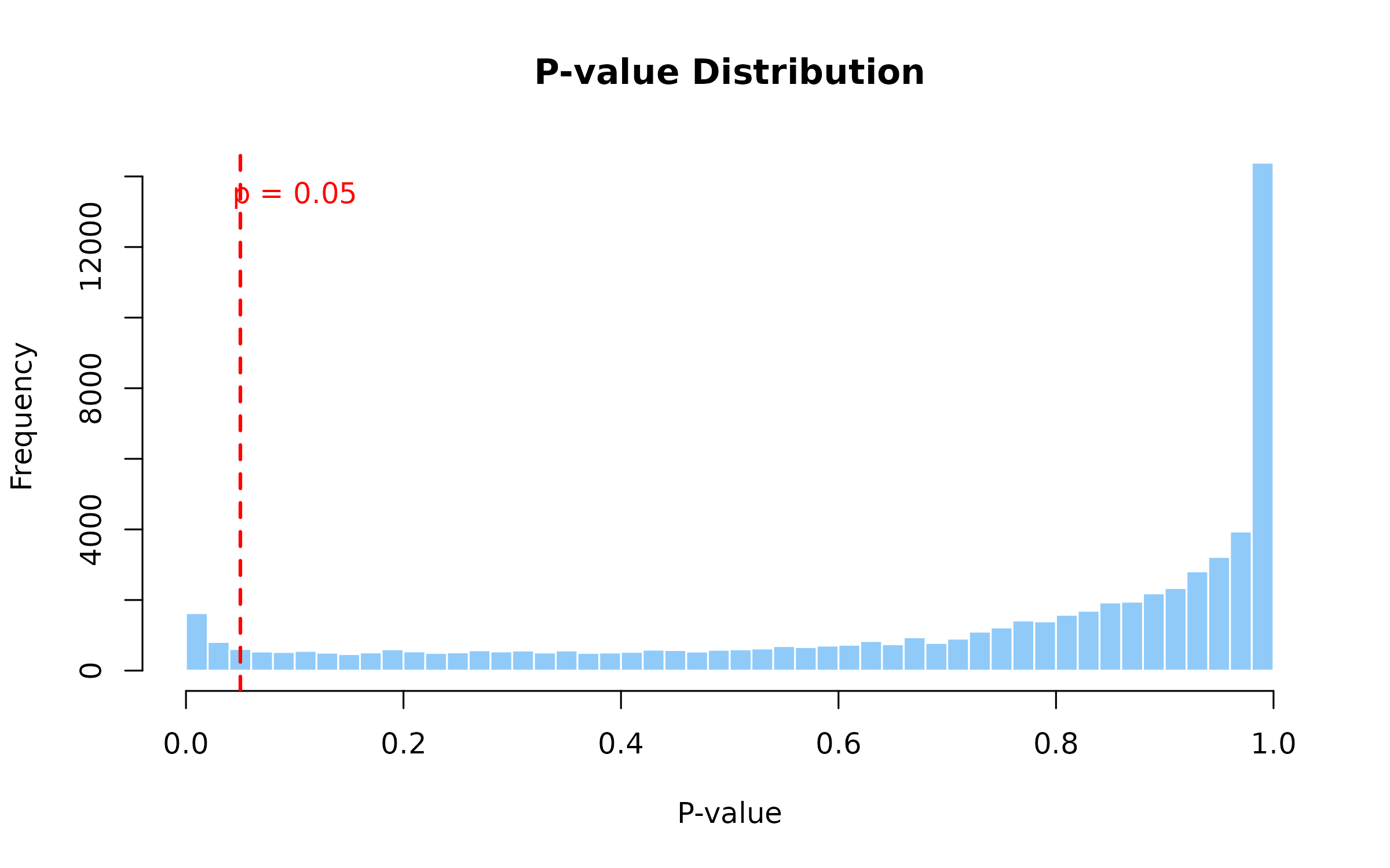
Figure 3: P-value Distribution from Permutation Test. Histogram of p-values from 100 permutations. A uniform distribution under the null is expected; enrichment near 0 indicates true signals. Red line marks the significance threshold (p=0.05).
Multiple Testing Correction
Different correction methods vary in stringency. With limited permutations (as in this tutorial), p-value correction may result in zero significant interactions:
# Different correction methods - show counts
obj_none <- filterSignificantInteractions(obj, adjust_method = "none")
obj_bh <- filterSignificantInteractions(obj, adjust_method = "BH")

cat("Significant interactions by correction method:\n")
#> Significant interactions by correction method:
cat("  No correction:", nrow(obj_none@significant_interactions), "\n")
#>   No correction: 2754
cat("  BH correction:", nrow(obj_bh@significant_interactions), "\n")
#> BH correction: 0Note: In real analysis with sufficient permutations (>1000), BH correction is recommended. For demonstration purposes with limited permutations, we use no adjustment.
Filtering Significant Interactions
# For this tutorial, use no adjustment to demonstrate the workflow
# In real analysis, use adjust_method = "BH" with more permutations
obj <- filterSignificantInteractions(
  obj,
  pvalue_threshold = 0.05, # Significance level
  adjust_method = "none", # Use "BH" for real analysis
  min_score = 0 # Minimum communication score
)

# View results
cat("Total significant interactions:", nrow(obj@significant_interactions), "\n\n")
#> Total significant interactions: 2754
cat("Top interactions:\n")
#> Top interactions:
head(obj@significant_interactions[, c(
  "sender", "receiver", "metabolite_name",
  "communication_score", "pvalue_adjusted"
)])
#>              sender receiver        metabolite_name communication_score
#> 1          Monocyte     Mast            Epinephrine           0.9999641
#> 2 Normal Epithelial   Plasma       5-Androstenediol           0.9992733
#> 3       Endothelial     Mast      Prostaglandin F1a           0.9903007
#> 4          Gliacyte        B 12-Keto-leukotriene B4           0.9862472
#> 5            Plasma   Plasma                Estriol           0.9822572
#> 6 Normal Macrophage        T    Cholesterol sulfate           0.9768051
#>   pvalue_adjusted
#> 1      0.00990099
#> 2      0.00990099
#> 3      0.00990099
#> 4      0.00990099
#> 5      0.00990099
#> 6      0.00990099
Exploring Communication Results
Communication Score Structure
# The communication_scores slot is a 3D array
comm <- obj@communication_scores
cat("Dimensions: sender x receiver x metabolite\n")
#> Dimensions: sender x receiver x metabolite
cat(dim(comm), "\n")
#> 15 15 286
cat("\nCell types:", dimnames(comm)[[1]], "\n")
#>
#> Cell types: Normal Epithelial T Plasma Normal Fibroblast CAF Normal Macrophage TAM B Monocyte Endothelial Pericyte SMC Mast Gliacyte Tumor Epithelial
cat("\nMetabolites (first 10):", head(dimnames(comm)[[3]], 10), "\n")
#>
#> Metabolites (first 10): HMDB0000010 HMDB0000011 HMDB0000015 HMDB0000016 HMDB0000031 HMDB0000034 HMDB0000036 HMDB0000039 HMDB0000042 HMDB0000045
Summarizing by Cell Type Pairs
# Different aggregation methods
sum_result <- summarizeCommunicationPairs(obj, aggregate_method = "sum")
mean_result <- summarizeCommunicationPairs(obj, aggregate_method = "mean")
count_result <- summarizeCommunicationPairs(obj, aggregate_method = "count")

cat("=== Sum of Communication Scores ===\n")
#> === Sum of Communication Scores ===
head(sum_result)
#>                sender          receiver communication_score
#> 128  Tumor Epithelial Normal Macrophage            52.63050
#> 199  Tumor Epithelial               TAM            51.99507
#> 191 Normal Epithelial               TAM            44.71782
#> 120 Normal Epithelial Normal Macrophage            43.56831
#> 106 Normal Epithelial Normal Fibroblast            40.51663
#> 30   Tumor Epithelial               CAF            37.72378

cat("\n=== Mean Communication Score ===\n")
#>
#> === Mean Communication Score ===
head(mean_result)
#>          sender receiver communication_score
#> 59  Endothelial     Mast           0.9903007
#> 62     Monocyte     Mast           0.8563538
#> 60     Gliacyte     Mast           0.8530255
#> 66     Pericyte     Mast           0.8407588
#> 132    Gliacyte Pericyte           0.8334445
#> 52     Pericyte Gliacyte           0.8238465

cat("\n=== Number of Significant Interactions ===\n")
#>
#> === Number of Significant Interactions ===
head(count_result)
#>                sender          receiver n_interactions
#> 128  Tumor Epithelial Normal Macrophage             82
#> 199  Tumor Epithelial               TAM             80
#> 106 Normal Epithelial Normal Fibroblast             69
#> 30   Tumor Epithelial               CAF             67
#> 113  Tumor Epithelial Normal Fibroblast             65
#> 191 Normal Epithelial               TAM             63
Get Communication Matrix
# Get aggregated communication matrix
comm_mat <- getCommunicationMatrix(obj, aggregate_method = "sum")

# Visualize
heatmap(comm_mat,
  col = hcl.colors(50, "Reds"),
  scale = "none",
  main = "Cell-Cell Communication Strength"
)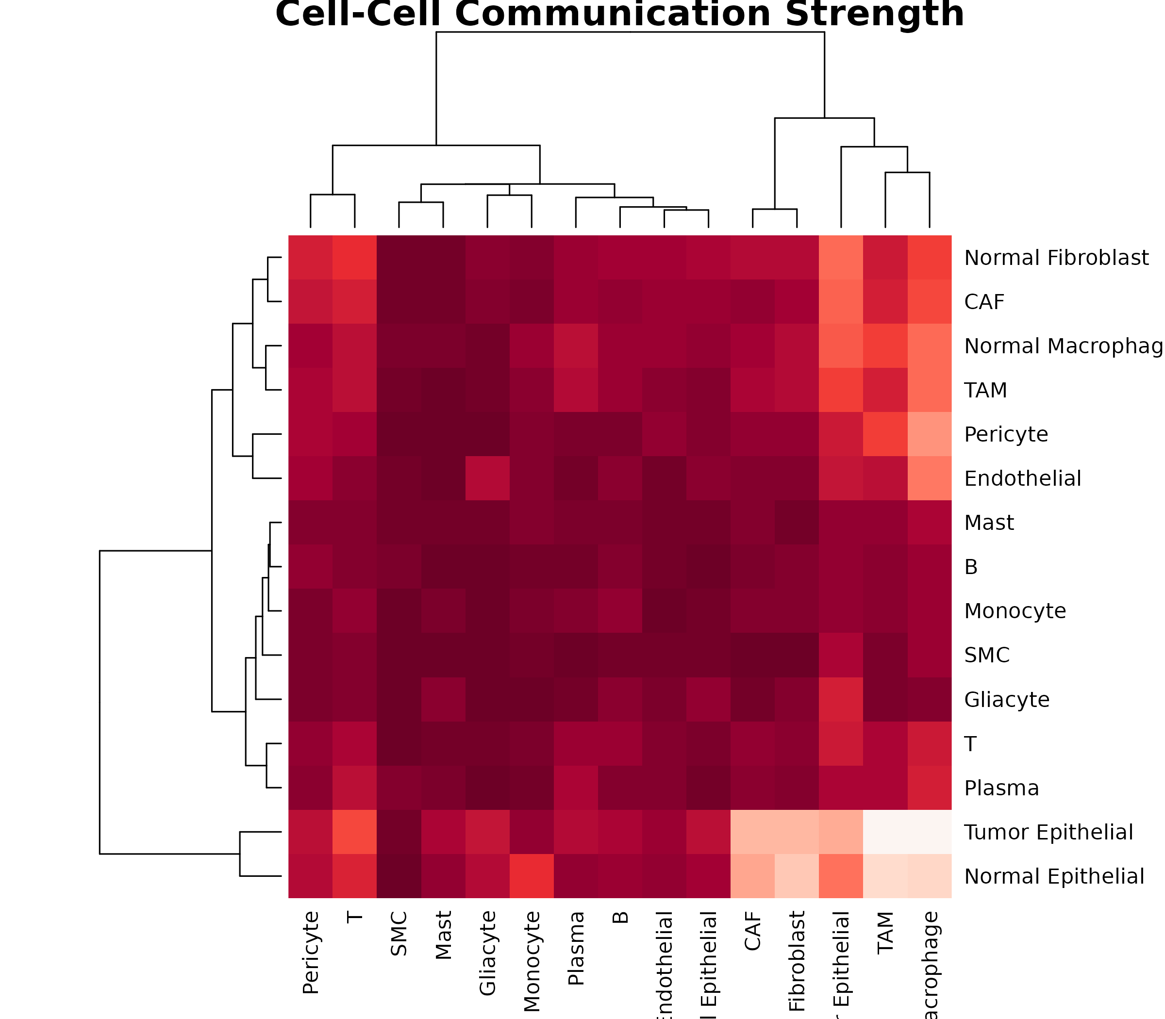
Figure 7: Cell-Cell Communication Matrix. Aggregated communication strength between all cell type pairs. Rows represent senders, columns represent receivers. Clustering groups cell types with similar communication patterns.
Analyzing Specific Interactions
Top Communicating Pairs
sig <- obj@significant_interactions

# Top sender-receiver pairs
pair_counts <- aggregate(communication_score ~ sender + receiver, data = sig, FUN = length)
names(pair_counts)[3] <- "n_metabolites"
pair_counts <- pair_counts[order(-pair_counts$n_metabolites), ]

cat("Top communicating cell type pairs:\n")
#> Top communicating cell type pairs:
head(pair_counts, 10)
#>                sender          receiver n_metabolites
#> 128  Tumor Epithelial Normal Macrophage            82
#> 199  Tumor Epithelial               TAM            80
#> 106 Normal Epithelial Normal Fibroblast            69
#> 30   Tumor Epithelial               CAF            67
#> 113  Tumor Epithelial Normal Fibroblast            65
#> 191 Normal Epithelial               TAM            63
#> 120 Normal Epithelial Normal Macrophage            61
#> 214  Tumor Epithelial  Tumor Epithelial            58
#> 22  Normal Epithelial               CAF            57
#> 123          Pericyte Normal Macrophage            47
Top Metabolite Mediators
# Most frequent metabolites in significant interactions
met_counts <- table(sig$metabolite_name)
met_counts <- sort(met_counts, decreasing = TRUE)

cat("Top metabolite mediators:\n")
#> Top metabolite mediators:
head(met_counts, 15)
#>
#> 11beta-Hydroxyprogesterone           5-Androstenediol
#>                         30                         23
#>                  Ornithine   7beta-Hydroxycholesterol
#>                         21                         20
#>    Adenosine monophosphate                  Cortisone
#>                         19                         19
#>                  Hydroxide                    Retinal
#>                         19                         18
#>                   L-Fucose     Uridine 5'-diphosphate
#>                         17                         17
#>                Cholesterol                   Cortisol
#>                         16                         16
#>                    Glycine             Hyocholic acid
#>                         16                         16
#>                  L-Proline
#>                         16
Specific Pathway Focus
# Filter for specific metabolites (e.g., amino acids)
amino_acids <- c(
  "L-Glutamic acid", "L-Glutamine", "L-Alanine", "Glycine",
  "L-Serine", "L-Proline", "L-Aspartic acid"
)

aa_interactions <- sig[sig$metabolite_name %in% amino_acids, ]
cat("Amino acid-mediated interactions:", nrow(aa_interactions), "\n\n")
#> Amino acid-mediated interactions: 90

if (nrow(aa_interactions) > 0) {
  # Summarize
  aa_summary <- aggregate(communication_score ~ sender + receiver + metabolite_name,
    data = aa_interactions, FUN = sum
  )
  aa_summary <- aa_summary[order(-aa_summary$communication_score), ]
  head(aa_summary, 10)
}
#>               sender          receiver metabolite_name communication_score
#> 32          Gliacyte  Tumor Epithelial L-Aspartic acid           0.8443290
#> 19 Normal Macrophage Normal Macrophage       L-Alanine           0.8136641
#> 75                 T            Plasma       L-Proline           0.8016842
#> 22               TAM Normal Macrophage       L-Alanine           0.7858833
#> 3  Normal Macrophage       Endothelial         Glycine           0.7542903
#> 57 Normal Macrophage               CAF     L-Glutamine           0.7450304
#> 60               TAM               CAF     L-Glutamine           0.7300418
#> 74            Plasma            Plasma       L-Proline           0.7230354
#> 62 Normal Macrophage Normal Fibroblast     L-Glutamine           0.7166993
#> 6                TAM       Endothelial         Glycine           0.7160865
Advanced: Directional Analysis
Outgoing Communication (as Sender)
# Which cell types send the most signals?
outgoing <- aggregate(communication_score ~ sender, data = sig, FUN = sum)
outgoing <- outgoing[order(-outgoing$communication_score), ]

barplot(outgoing$communication_score,
  names.arg = outgoing$sender,
  las = 2, col = "#FF7043",
  main = "Outgoing Communication Strength",
  ylab = "Total Communication Score"
)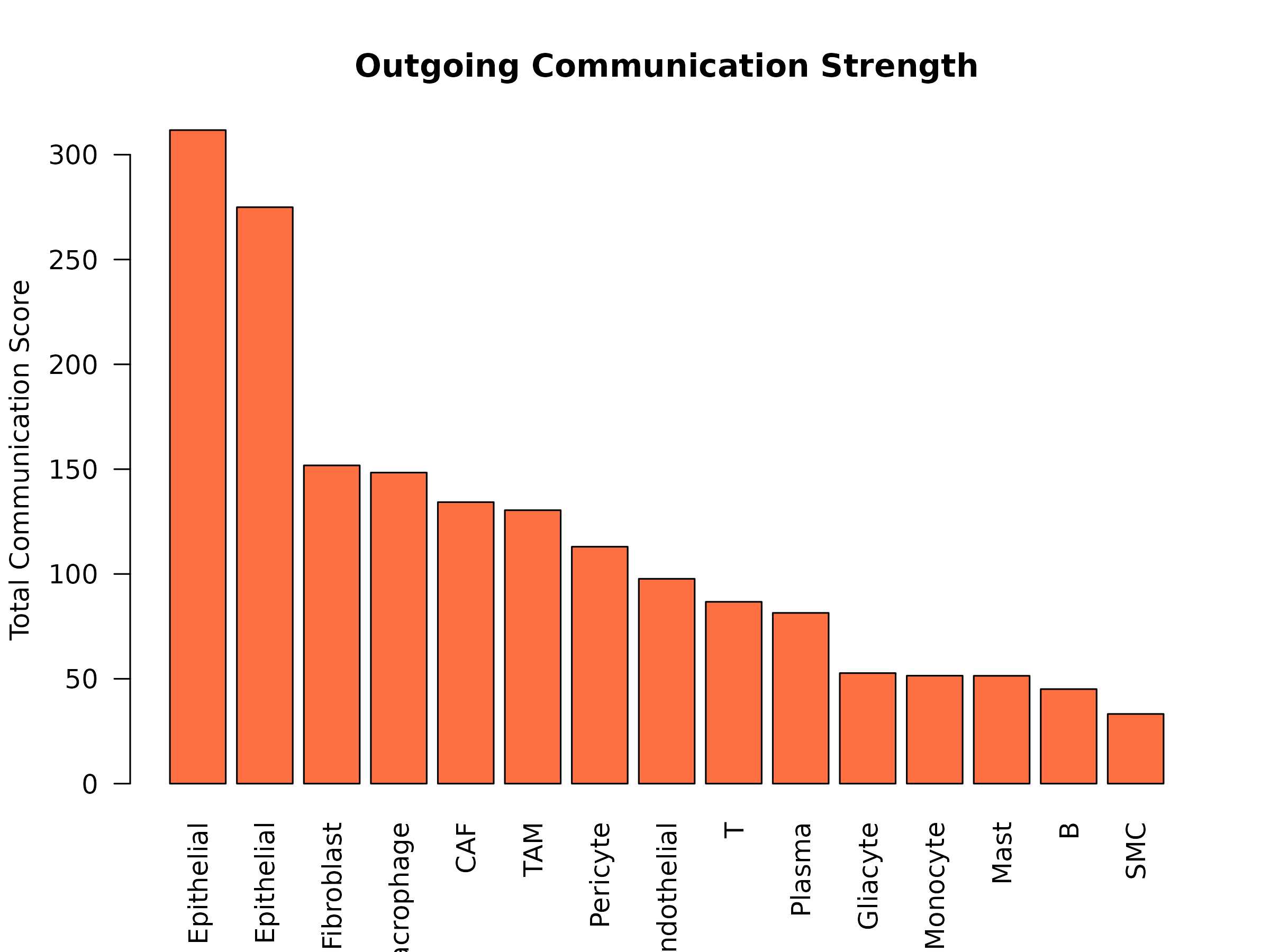
Figure 4: Outgoing Communication Strength. Total communication scores for each cell type acting as a sender. Higher values indicate cell types that produce more metabolites for intercellular signaling.
Incoming Communication (as Receiver)
# Which cell types receive the most signals?
incoming <- aggregate(communication_score ~ receiver, data = sig, FUN = sum)
incoming <- incoming[order(-incoming$communication_score), ]

barplot(incoming$communication_score,
  names.arg = incoming$receiver,
  las = 2, col = "#42A5F5",
  main = "Incoming Communication Strength",
  ylab = "Total Communication Score"
)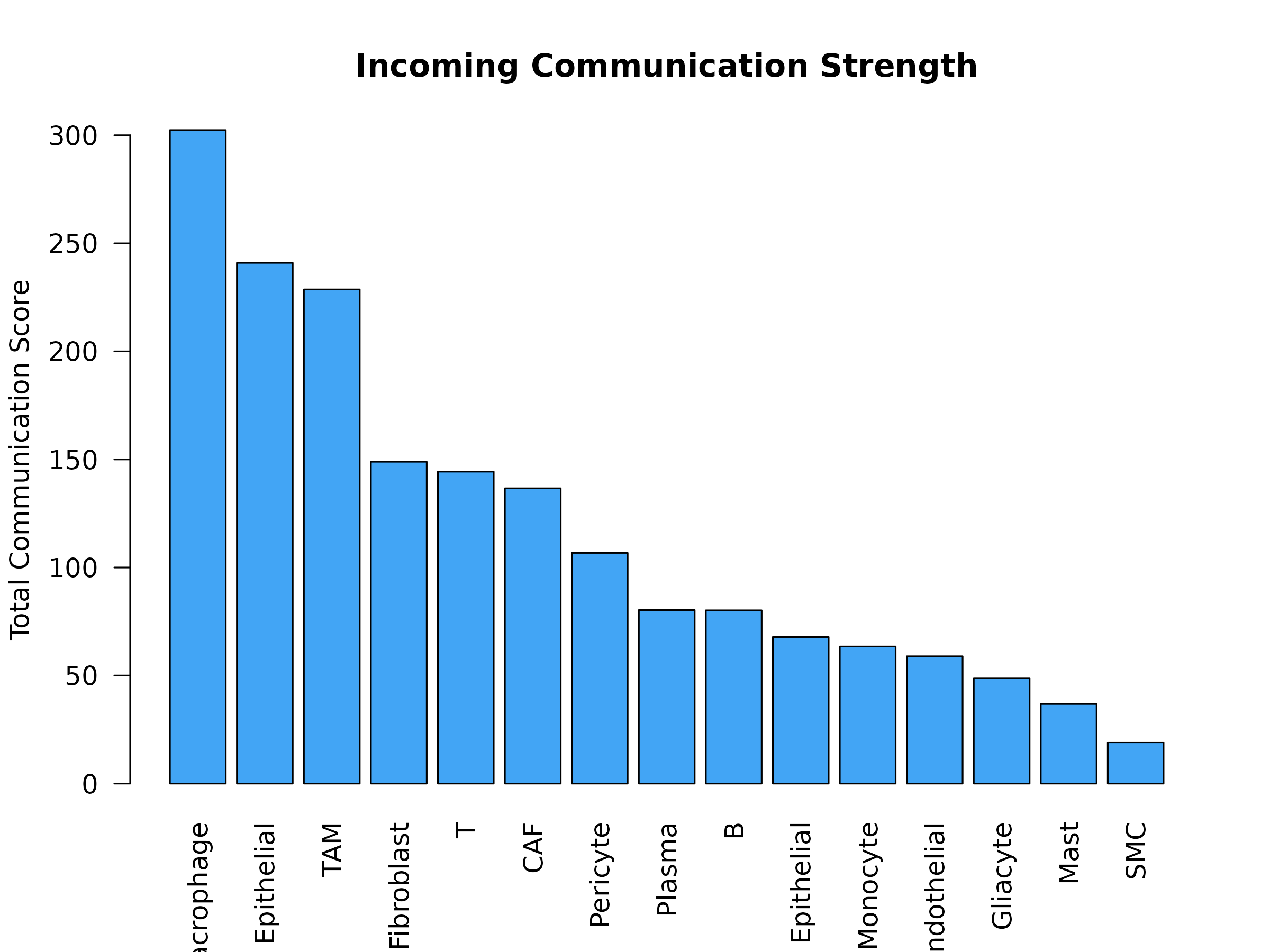
Figure 5: Incoming Communication Strength. Total communication scores for each cell type acting as a receiver. Higher values indicate cell types that sense/uptake more metabolites from other cells.
Net Communication Flow
# Net flow = Outgoing - Incoming
cell_types <- unique(c(sig$sender, sig$receiver))
net_flow <- sapply(cell_types, function(ct) {
  out <- sum(sig$communication_score[sig$sender == ct])
  inc <- sum(sig$communication_score[sig$receiver == ct])
  out - inc
})

# Sort and plot
net_flow <- sort(net_flow, decreasing = TRUE)
cols <- ifelse(net_flow > 0, "#FF7043", "#42A5F5")

barplot(net_flow,
  col = cols, las = 2,
  main = "Net Communication Flow",
  ylab = "Outgoing - Incoming"
)
abline(h = 0, lty = 2)
legend("topright",
  legend = c("Net Sender", "Net Receiver"),
  fill = c("#FF7043", "#42A5F5")
)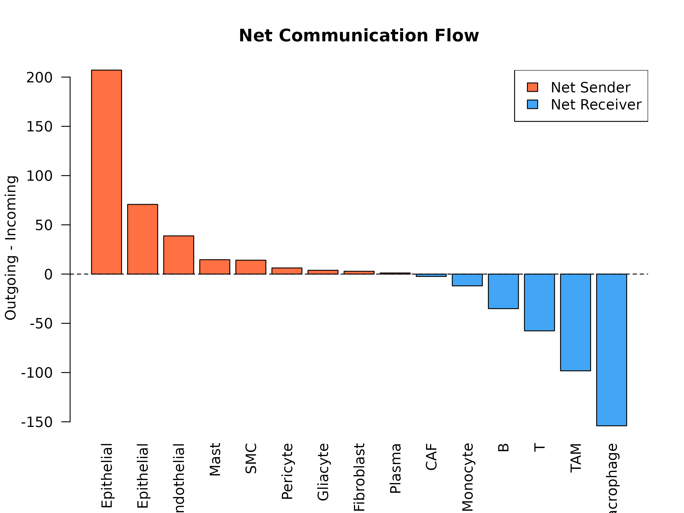
Figure 6: Net Communication Flow. Difference between outgoing and incoming communication for each cell type. Positive values (orange) indicate net senders; negative values (blue) indicate net receivers. This reveals which cell types drive vs receive metabolic signals in the tissue.
Comparing Conditions (If Available)
# If your data has conditions (e.g., tumor vs normal)
# You can run scMetaLink separately and compare

# Example workflow:
obj_tumor <- runScMetaLink(expr_tumor, meta_tumor, "cell_type")
obj_normal <- runScMetaLink(expr_normal, meta_normal, "cell_type")

# Compare communication strength
comm_tumor <- getCommunicationMatrix(obj_tumor)
comm_normal <- getCommunicationMatrix(obj_normal)

# Differential communication
diff_comm <- comm_tumor - comm_normal
Output Summary
| Output | Description | Access |
|---|---|---|
| Communication scores | 3D array (sender x receiver x metabolite) | obj@communication_scores |
| P-values | 3D array of permutation p-values | obj@communication_pvalues |
| Significant interactions | Filtered data.frame | obj@significant_interactions |
| Summary matrix | 2D aggregated matrix | getCommunicationMatrix(obj) |
| Pair summary | data.frame by cell type pairs | summarizeCommunicationPairs(obj) |
Next Steps
- Spatial Analysis: Spatial transcriptomics support
- Visualization: Create publication-ready figures
- Applications: Real-world analysis examples