Overview
scMetaLink provides a specialized module for analyzing lactate-mediated cell communication. Lactate is not merely a metabolic waste product but a critical signaling molecule in the tumor microenvironment (TME). This module captures both direct and indirect lactate signaling pathways based on rigorous scientific literature review.
Scientific Background
The Dual Role of Lactate
Lactate exerts its signaling effects through two distinct mechanisms:
- Direct Signaling: Lactate directly binds to HCAR1 (GPR81), the only confirmed lactate GPCR
- Indirect Signaling: Lactate dissociation (pKa=3.86) produces H+ ions that activate proton-sensing GPCRs
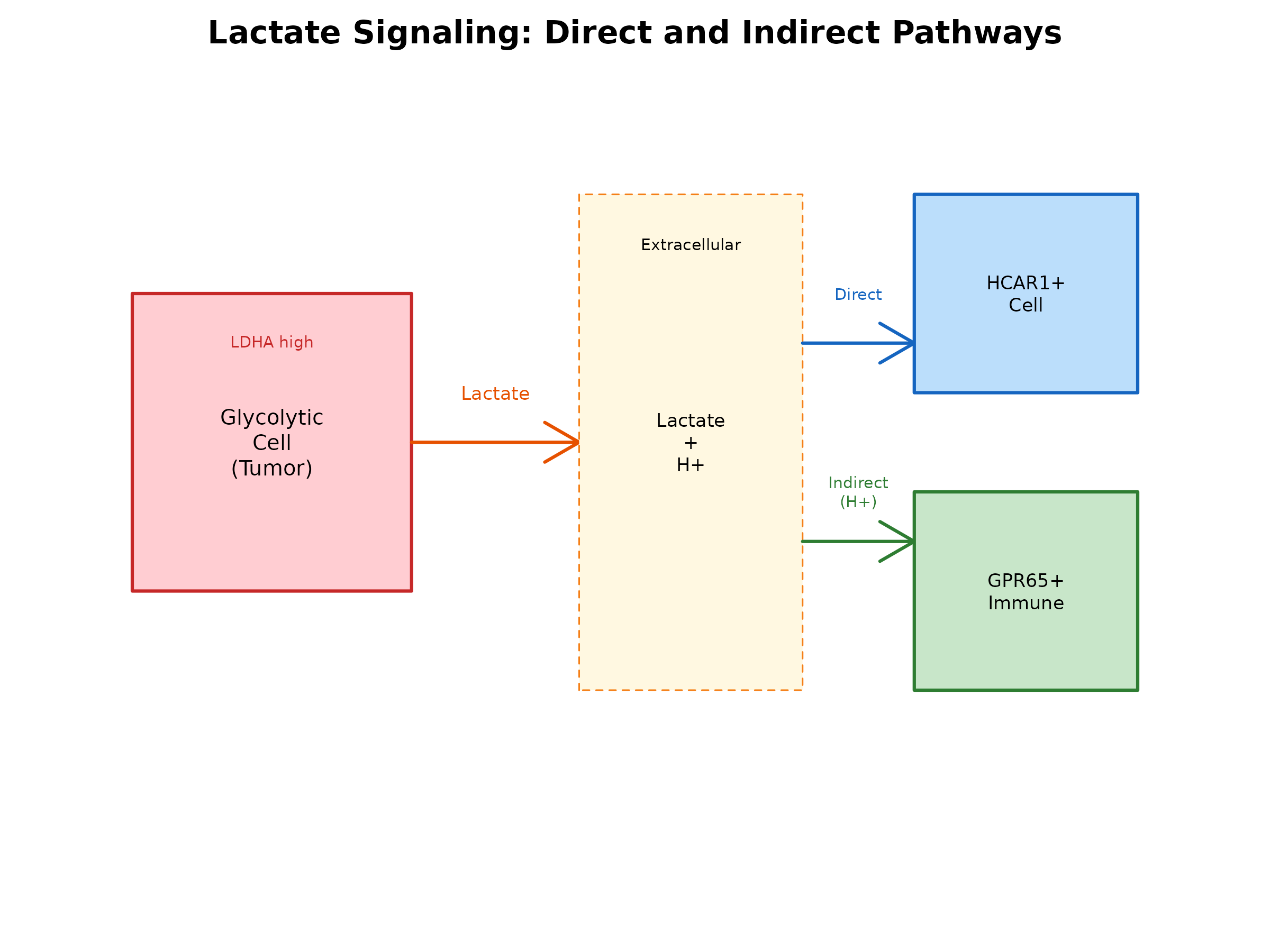
Figure 1: Lactate Signaling Pathways. Lactate produced by glycolytic cells (e.g., tumor cells) can signal through direct binding to HCAR1 or indirectly through H+ activation of proton-sensing GPCRs.
Key Biological Facts
| Aspect | Details | Evidence |
|---|---|---|
| Lactate pKa | 3.86 (nearly 100% dissociated at pH 7.4) | Chemical property |
| Direct receptor | HCAR1 (GPR81) - only confirmed lactate GPCR | PLOS Biology 2024 |
| Proton sensors | GPR4, GPR65, GPR68, GPR132 | Reactome R-HSA-444731 |
| Primary exporter | MCT4 (SLC16A3) - low affinity, glycolytic cells | iScience 2019 |
| Primary importer | MCT1 (SLC16A1) - high affinity, oxidative cells | Nature 2025 |
| MCT chaperone | BSG/CD147 - essential for membrane localization | Nature 2025 |
Load Data and Run Analysis
library(scMetaLink)
library(Matrix)

# Load built-in colorectal cancer example data
data(crc_example)

# Create scMetaLink object
obj <- createScMetaLink(crc_expr, crc_meta, "cell_type")

cat("Cell types in data:\n")
#> Cell types in data:
print(table(crc_meta$cell_type))
#>
#>                 B               CAF       Endothelial          Gliacyte
#>               150               200               100                20
#>              Mast          Monocyte Normal Epithelial Normal Fibroblast
#>                30               120               300               200
#> Normal Macrophage          Pericyte            Plasma               SMC
#>               150                50               250                30
#>                 T               TAM  Tumor Epithelial
#>               500               150               600
Gene Sets
The lactate module uses scientifically curated gene sets:
# Get all gene sets
genes <- getLactateGenes()

cat("=== PRODUCTION ===\n")
#> === PRODUCTION ===
cat("Synthesis enzymes:\n")
#> Synthesis enzymes:
print(genes$production$synthesis)
#> [1] "LDHA"    "LDHC"    "LDHAL6A" "LDHAL6B"
cat("\nExport transporters:\n")
#>
#> Export transporters:
print(genes$production$export)
#> [1] "SLC16A3" "SLC16A1" "SLC16A7" "SLC16A8" "AQP9"    "BSG"

cat("\n=== DEGRADATION ===\n")
#>
#> === DEGRADATION ===
print(genes$degradation$enzymes)
#> [1] "LDHB" "LDHD"

cat("\n=== DIRECT SENSING ===\n")
#>
#> === DIRECT SENSING ===
print(genes$direct_sensing$receptor)
#> [1] "HCAR1"

cat("\n=== INDIRECT SENSING (Proton GPCRs) ===\n")
#>
#> === INDIRECT SENSING (Proton GPCRs) ===
print(genes$indirect_sensing$proton_receptors)
#> [1] "GPR4"   "GPR65"  "GPR68"  "GPR132"
cat("Weights (reflecting pH sensitivity):\n")
#> Weights (reflecting pH sensitivity):
print(genes$indirect_sensing$weights)
#>   GPR4  GPR65  GPR68 GPR132
#>    1.0    1.0    1.0    0.5

cat("\n=== UPTAKE ===\n")
#>
#> === UPTAKE ===
print(genes$uptake$import)
#> [1] "SLC16A1" "SLC16A7" "BSG"
Why These Genes?
Production (Synthesis): - LDHA is the primary enzyme catalyzing pyruvate → lactate (Warburg effect) - LDHB is excluded because it preferentially catalyzes the reverse reaction
Production (Export): - MCT4 (SLC16A3) is the primary exporter with low affinity (Km ~22-28 mM) - BSG/CD147 is an essential chaperone required for MCT membrane localization
Direct Sensing: - HCAR1 is the only confirmed lactate GPCR (validated by cryo-EM structure in 2024)
Indirect Sensing: - Classic proton-sensing GPCRs that detect pH via histidine protonation - GPR132 has reduced weight (0.5) because it primarily senses oxidized fatty acids
Check Gene Availability
Before running analysis, check which lactate genes are available in your data:
# Check gene availability (returns a data.frame with category, subcategory, gene, available)
gene_check <- checkLactateGenes(obj)
#> Lactate Gene Availability Summary:
#> ==================================
#>          category    available
#>       degradation   2/2 (100%)
#>    direct_sensing   1/1 (100%)
#>  indirect_sensing   4/4 (100%)
#>        production 10/10 (100%)
#>            uptake   3/3 (100%)

# Visualize gene availability by category
categories <- c("Production", "Degradation", "Direct Sensing", "Indirect Sensing", "Uptake")
category_keys <- c("production", "degradation", "direct_sensing", "indirect_sensing", "uptake")

available <- sapply(category_keys, function(cat) {
  sum(gene_check$available[gene_check$category == cat])
})
total <- sapply(category_keys, function(cat) {
  sum(gene_check$category == cat)
})

par(mar = c(5, 8, 4, 2))
barplot(rbind(available, total - available),
        beside = FALSE, horiz = TRUE,
        names.arg = categories, las = 1,
        col = c("#4CAF50", "#FFCDD2"),
        main = "Lactate Gene Availability",
        xlab = "Number of Genes")
legend("bottomright", c("Available", "Missing"), fill = c("#4CAF50", "#FFCDD2"))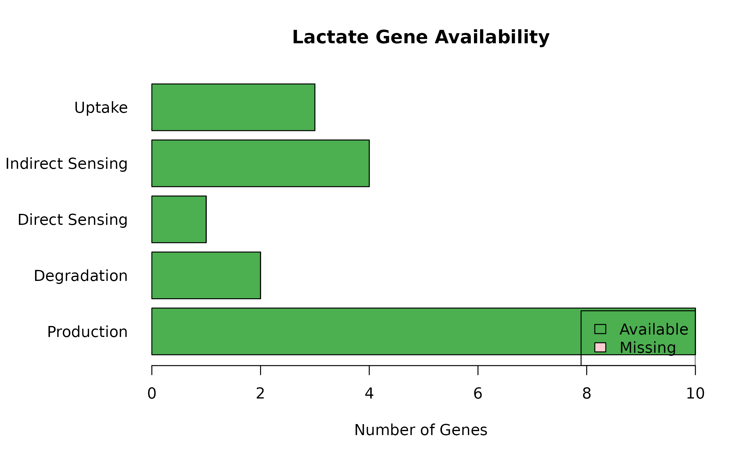
Figure 2: Lactate Gene Availability. Presence of lactate-related genes in the dataset.
Run Lactate Signaling Analysis
# Run full lactate signaling analysis
obj <- inferLactateSignaling(
obj,
include_direct = TRUE,
include_indirect = TRUE,
method = "combined",
normalize = TRUE,
n_permutations = 100, # Use more for real analysis
verbose = TRUE
)
#> | | | 0% | |= | 1% | |= | 2% | |== | 3% | |=== | 4% | |==== | 5% | |==== | 6% | |===== | 7% | |====== | 8% | |====== | 9% | |======= | 10% | |======== | 11% | |======== | 12% | |========= | 13% | |========== | 14% | |========== | 15% | |=========== | 16% | |============ | 17% | |============= | 18% | |============= | 19% | |============== | 20% | |=============== | 21% | |=============== | 22% | |================ | 23% | |================= | 24% | |================== | 25% | |================== | 26% | |=================== | 27% | |==================== | 28% | |==================== | 29% | |===================== | 30% | |====================== | 31% | |====================== | 32% | |======================= | 33% | |======================== | 34% | |======================== | 35% | |========================= | 36% | |========================== | 37% | |=========================== | 38% | |=========================== | 39% | |============================ | 40% | |============================= | 41% | |============================= | 42% | |============================== | 43% | |=============================== | 44% | |================================ | 45% | |================================ | 46% | |================================= | 47% | |================================== | 48% | |================================== | 49% | |=================================== | 50% | |==================================== | 51% | |==================================== | 52% | |===================================== | 53% | |====================================== | 54% | |====================================== | 55% | |======================================= | 56% | |======================================== | 57% | |========================================= | 58% | |========================================= | 59% | |========================================== | 60% | |=========================================== | 61% | |=========================================== | 62% | |============================================ | 63% | |============================================= | 64% | |============================================== | 65% | |============================================== | 66% | |=============================================== | 67% | |================================================ | 68% | |================================================ | 69% | |================================================= | 70% | |================================================== | 71% | |================================================== | 72% | |=================================================== | 73% | |==================================================== | 74% | |==================================================== | 75% | |===================================================== | 76% | |====================================================== | 77% | |======================================================= | 78% | |======================================================= | 79% | |======================================================== | 80% | |========================================================= | 81% | |========================================================= | 82% | |========================================================== | 83% | |=========================================================== | 84% | |============================================================ | 85% | |============================================================ | 86% | |============================================================= | 87% | |============================================================== | 88% | |============================================================== | 89% | |=============================================================== | 90% | |================================================================ | 91% | |================================================================ | 92% | |================================================================= | 93% | |================================================================== | 94% | |================================================================== | 95% | |=================================================================== | 96% | |==================================================================== | 97% | |===================================================================== | 98% | |===================================================================== | 99% | |======================================================================| 100%
#> | | | 0% | |= | 1% | |= | 2% | |== | 3% | |=== | 4% | |==== | 5% | |==== | 6% | |===== | 7% | |====== | 8% | |====== | 9% | |======= | 10% | |======== | 11% | |======== | 12% | |========= | 13% | |========== | 14% | |========== | 15% | |=========== | 16% | |============ | 17% | |============= | 18% | |============= | 19% | |============== | 20% | |=============== | 21% | |=============== | 22% | |================ | 23% | |================= | 24% | |================== | 25% | |================== | 26% | |=================== | 27% | |==================== | 28% | |==================== | 29% | |===================== | 30% | |====================== | 31% | |====================== | 32% | |======================= | 33% | |======================== | 34% | |======================== | 35% | |========================= | 36% | |========================== | 37% | |=========================== | 38% | |=========================== | 39% | |============================ | 40% | |============================= | 41% | |============================= | 42% | |============================== | 43% | |=============================== | 44% | |================================ | 45% | |================================ | 46% | |================================= | 47% | |================================== | 48% | |================================== | 49% | |=================================== | 50% | |==================================== | 51% | |==================================== | 52% | |===================================== | 53% | |====================================== | 54% | |====================================== | 55% | |======================================= | 56% | |======================================== | 57% | |========================================= | 58% | |========================================= | 59% | |========================================== | 60% | |=========================================== | 61% | |=========================================== | 62% | |============================================ | 63% | |============================================= | 64% | |============================================== | 65% | |============================================== | 66% | |=============================================== | 67% | |================================================ | 68% | |================================================ | 69% | |================================================= | 70% | |================================================== | 71% | |================================================== | 72% | |=================================================== | 73% | |==================================================== | 74% | |==================================================== | 75% | |===================================================== | 76% | |====================================================== | 77% | |======================================================= | 78% | |======================================================= | 79% | |======================================================== | 80% | |========================================================= | 81% | |========================================================= | 82% | |========================================================== | 83% | |=========================================================== | 84% | |============================================================ | 85% | |============================================================ | 86% | |============================================================= | 87% | |============================================================== | 88% | |============================================================== | 89% | |=============================================================== | 90% | |================================================================ | 91% | |================================================================ | 92% | |================================================================= | 93% | |================================================================== | 94% | |================================================================== | 95% | |=================================================================== | 96% | |==================================================================== | 97% | |===================================================================== | 98% | |===================================================================== | 99% | |======================================================================| 100%Visualize Results
Production Scores
# Get lactate results
lactate_results <- obj@parameters$lactate_signaling

if (!is.null(lactate_results)) {
  prod_scores <- lactate_results$production

  # Sort and plot
  prod_sorted <- sort(prod_scores, decreasing = TRUE)

  par(mar = c(5, 10, 4, 2))
  barplot(prod_sorted, horiz = TRUE, las = 1,
          col = "#FF7043", border = NA,
          main = "Lactate Production by Cell Type",
          xlab = "Production Score")
}
Figure 3: Lactate Production Scores. Higher scores indicate greater lactate production potential (high LDHA, MCT4 expression).
Sensing Scores Comparison
if (!is.null(lactate_results)) {
  direct_sens <- lactate_results$direct_sensing
  indirect_sens <- lactate_results$indirect_sensing

  # Combine for plotting
  cell_types <- names(direct_sens)

  par(mar = c(5, 10, 4, 2))

  # Create grouped barplot
  sens_mat <- rbind(Direct = direct_sens, Indirect = indirect_sens)

  barplot(sens_mat, beside = TRUE, horiz = TRUE, las = 1,
          col = c("#1565C0", "#2E7D32"), border = NA,
          main = "Lactate Sensing: Direct vs Indirect Pathways",
          xlab = "Sensing Score")
  legend("bottomright", c("Direct (HCAR1)", "Indirect (H+/GPCRs)"),
         fill = c("#1565C0", "#2E7D32"), bty = "n")
}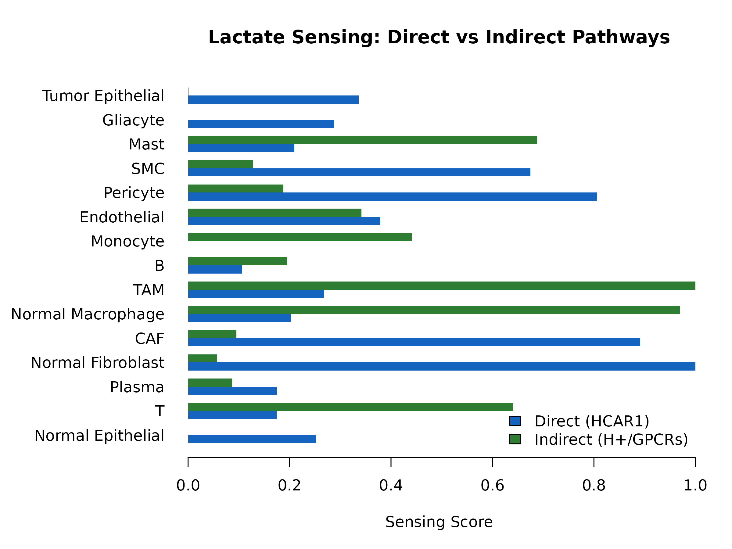
Figure 4: Lactate Sensing Scores. Comparison of direct (HCAR1) vs indirect (proton GPCRs) sensing across cell types.
Communication Heatmap
if (!is.null(lactate_results) && !is.null(lactate_results$combined_communication)) {
  # Plot using the built-in function
  plotLactateSignaling(obj, pathway = "combined")
}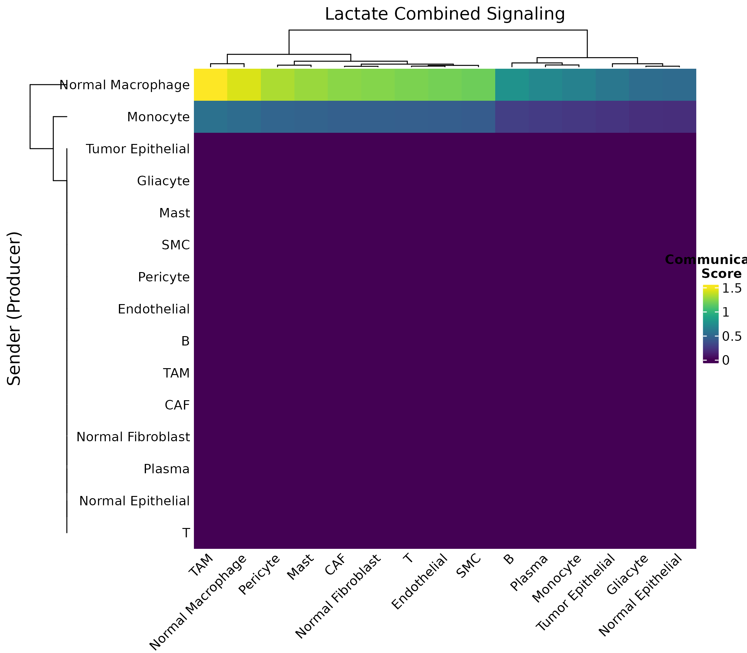
Figure 5: Lactate Communication Heatmap. Communication strength from sender (rows) to receiver (columns) cell types via lactate signaling.
Pathway Comparison
if (!is.null(lactate_results)) {
  plotLactatePathwayComparison(obj, show_production = TRUE)
}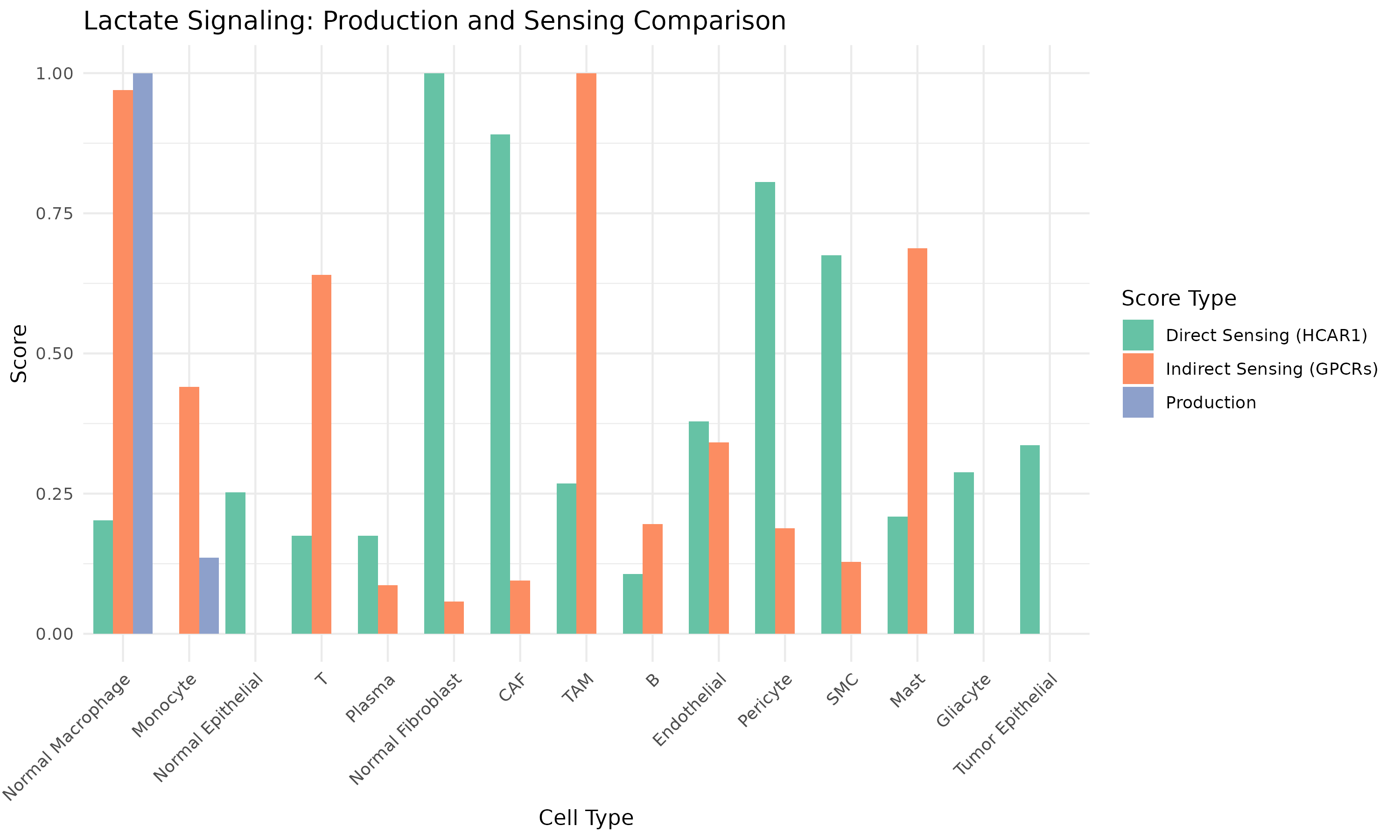
Figure 6: Production vs Sensing Comparison. Cell types positioned by their lactate production (orange) and sensing (blue) capabilities.
Cell Type Roles
if (!is.null(lactate_results) && !is.null(lactate_results$combined_communication)) {
  comm <- lactate_results$combined_communication

  # Calculate net flow
  cell_types <- rownames(comm)
  net_flow <- rowSums(comm) - colSums(comm)
  net_flow <- sort(net_flow)

  par(mar = c(5, 10, 4, 2))
  cols <- ifelse(net_flow > 0, "#FF7043", "#42A5F5")
  barplot(net_flow, horiz = TRUE, las = 1,
          col = cols, border = NA,
          main = "Net Lactate Communication Flow",
          xlab = "Net Flow (Outgoing - Incoming)")
  abline(v = 0, lty = 2, col = "gray50")
  legend("bottomright", c("Net Producer", "Net Sensor"),
         fill = c("#FF7043", "#42A5F5"), bty = "n")
}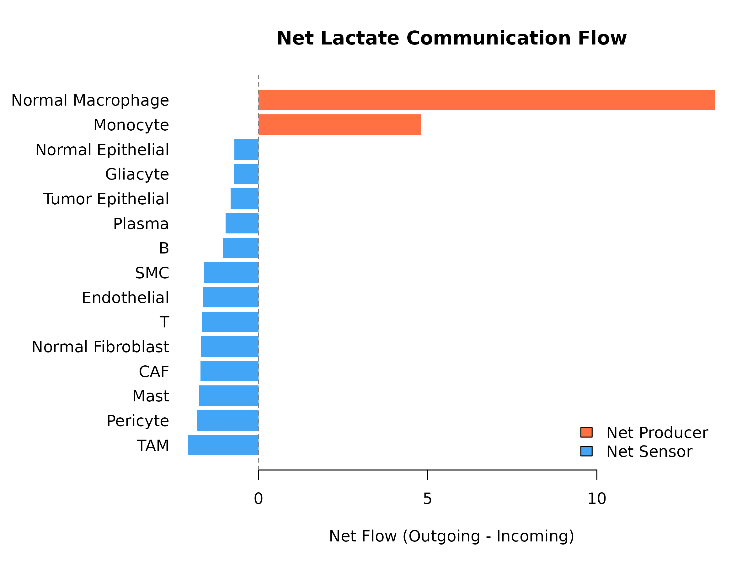
Figure 7: Cell Type Metabolic Roles in Lactate Signaling. Net lactate flow: positive = net producer, negative = net sensor.
Interpreting Results
Production Scores
High production indicates: - High expression of LDHA (synthesis) - High expression of MCT4/BSG (export) - Low expression of LDHB (degradation)
Sensing Scores
Direct pathway (HCAR1): - Indicates cells that can directly respond to lactate - Important in anti-inflammatory signaling
Indirect pathway (H+/proton GPCRs): - Indicates cells sensing acidification from lactate dissociation - Critical for immune cell function in TME
Top Communicators
if (!is.null(lactate_results)) {
  summary_df <- getLactateSignalingSummary(obj, pathway = "combined", top_n = 10)
  print(summary_df)
}
#>               sender          receiver communication_score rank
#> 1  Normal Macrophage               TAM           1.5176455    1
#> 2  Normal Macrophage Normal Macrophage           1.4345244    2
#> 3  Normal Macrophage          Pericyte           1.3311660    3
#> 4  Normal Macrophage              Mast           1.2868515    4
#> 5  Normal Macrophage               CAF           1.2522300    5
#> 6  Normal Macrophage Normal Fibroblast           1.2392587    6
#> 7  Normal Macrophage                 T           1.2179554    7
#> 8  Normal Macrophage       Endothelial           1.2001152    8
#> 9  Normal Macrophage               SMC           1.1799733    9
#> 10 Normal Macrophage                 B           0.7686704   10
Algorithm Details
Production Score
Where: - Synthesis = {LDHA, LDHC, LDHAL6A, LDHAL6B} - Export = {SLC16A3, SLC16A1, SLC16A7, SLC16A8, AQP9, BSG} - Degradation = {LDHB, LDHD} - α = 0.3 (degradation weight)
Biological Applications
References
- HCAR1/GPR81 Structure: PLOS Biology (2024). Cryo-EM structures of HCAR1.
- GPR81 Function: Nature Metabolism (2024). Lactate drives cachexia via GPR81.
- MCT Transport: iScience (2019). Role of MCT4 in lactate shuttle.
- BSG/CD147: Nature Cell Discovery (2025). Basigin modulates MCTs.
- Proton GPCRs: Reactome R-HSA-444731.
See Also
- Quick Start: Getting started with scMetaLink
- Theory & Methods: Mathematical framework
- Spatial Analysis: Spatial transcriptomics support
- Visualization: Complete visualization guide
Session Info
sessionInfo()
#> R version 4.5.2 (2025-10-31)
#> Platform: x86_64-pc-linux-gnu
#> Running under: Ubuntu 24.04.3 LTS
#>
#> Matrix products: default
#> BLAS:   /usr/lib/x86_64-linux-gnu/openblas-pthread/libblas.so.3
#> LAPACK: /usr/lib/x86_64-linux-gnu/openblas-pthread/libopenblasp-r0.3.26.so;  LAPACK version 3.12.0
#>
#> locale:
#>  [1] LC_CTYPE=C.UTF-8       LC_NUMERIC=C           LC_TIME=C.UTF-8
#>  [4] LC_COLLATE=C.UTF-8     LC_MONETARY=C.UTF-8    LC_MESSAGES=C.UTF-8
#>  [7] LC_PAPER=C.UTF-8       LC_NAME=C              LC_ADDRESS=C
#> [10] LC_TELEPHONE=C         LC_MEASUREMENT=C.UTF-8 LC_IDENTIFICATION=C
#>
#> time zone: UTC
#> tzcode source: system (glibc)
#>
#> attached base packages:
#> [1] stats     graphics  grDevices utils     datasets  methods   base
#>
#> other attached packages:
#> [1] Matrix_1.7-4      scMetaLink_0.99.0
#>
#> loaded via a namespace (and not attached):
#>  [1] viridis_0.6.5         sass_0.4.10           generics_0.1.4
#>  [4] shape_1.4.6.1         lattice_0.22-7        digest_0.6.39
#>  [7] magrittr_2.0.4        evaluate_1.0.5        grid_4.5.2
#> [10] RColorBrewer_1.1-3    iterators_1.0.14      circlize_0.4.17
#> [13] fastmap_1.2.0         foreach_1.5.2         doParallel_1.0.17
#> [16] jsonlite_2.0.0        GlobalOptions_0.1.3   gridExtra_2.3
#> [19] ComplexHeatmap_2.26.0 viridisLite_0.4.2     scales_1.4.0
#> [22] codetools_0.2-20      textshaping_1.0.4     jquerylib_0.1.4
#> [25] cli_3.6.5             rlang_1.1.7           crayon_1.5.3
#> [28] withr_3.0.2           cachem_1.1.0          yaml_2.3.12
#> [31] otel_0.2.0            tools_4.5.2           parallel_4.5.2
#> [34] dplyr_1.1.4           colorspace_2.1-2      ggplot2_4.0.1
#> [37] BiocGenerics_0.56.0   GetoptLong_1.1.0      vctrs_0.7.0
#> [40] R6_2.6.1              png_0.1-8             stats4_4.5.2
#> [43] matrixStats_1.5.0     lifecycle_1.0.5       S4Vectors_0.48.0
#> [46] IRanges_2.44.0        fs_1.6.6              htmlwidgets_1.6.4
#> [49] clue_0.3-66           cluster_2.1.8.1       ragg_1.5.0
#> [52] pkgconfig_2.0.3       desc_1.4.3            pkgdown_2.2.0
#> [55] pillar_1.11.1         bslib_0.9.0           gtable_0.3.6
#> [58] glue_1.8.0            systemfonts_1.3.1     xfun_0.56
#> [61] tibble_3.3.1          tidyselect_1.2.1      knitr_1.51
#> [64] farver_2.1.2          rjson_0.2.23          htmltools_0.5.9
#> [67] labeling_0.4.3        rmarkdown_2.30        compiler_4.5.2
#> [70] S7_0.2.1