Introduction
scMetaLink infers metabolite-mediated cell-cell communication from single-cell RNA-seq data. Unlike traditional ligand-receptor analysis, scMetaLink focuses on metabolites as signaling mediators, capturing a crucial but often overlooked layer of intercellular communication.
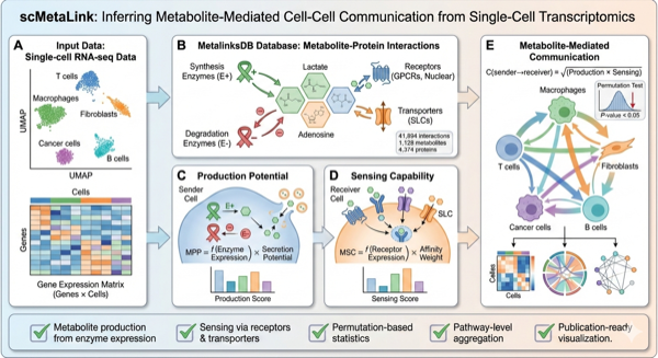
Figure 1: scMetaLink Workflow. Overview of the scMetaLink analysis pipeline.
Load Package and Example Data
library(scMetaLink)
library(Matrix)

# Load built-in colorectal cancer example data
data(crc_example)

# Check the data structure
cat("Expression matrix dimensions:", dim(crc_expr), "\n")
#> Expression matrix dimensions: 4210 2850
cat("Genes:", nrow(crc_expr), "| Cells:", ncol(crc_expr), "\n")
#> Genes: 4210 | Cells: 2850
cat("\nCell metadata:\n")
#>
#> Cell metadata:
head(crc_meta)
#>                   cell_type tumor_normal   tissue_region
#> Cell_0001 Normal Epithelial       Normal Normal Adjacent
#> Cell_0002 Normal Epithelial       Normal Normal Adjacent
#> Cell_0003 Normal Epithelial       Normal Normal Adjacent
#> Cell_0004 Normal Epithelial       Normal Normal Adjacent
#> Cell_0005 Normal Epithelial       Normal Normal Adjacent
#> Cell_0006 Normal Epithelial       Normal Normal Adjacent
cat("\nCell type distribution:\n")
#>
#> Cell type distribution:
print(table(crc_meta$cell_type))
#>
#>                 B               CAF       Endothelial          Gliacyte
#>               150               200               100                20
#>              Mast          Monocyte Normal Epithelial Normal Fibroblast
#>                30               120               300               200
#> Normal Macrophage          Pericyte            Plasma               SMC
#>               150                50               250                30
#>                 T               TAM  Tumor Epithelial
#>               500               150               600
The 5-Minute Workflow
Step 1: Create scMetaLink Object
# Create the analysis object
obj <- createScMetaLink(
  expression_data = crc_expr,
  cell_meta = crc_meta,
  cell_type_column = "cell_type"
)

# Check the object
obj
#> scMetaLink Object
#> =================
#> Genes: 4210
#> Cells: 2850
#> Cell types: 15 (Normal Epithelial, T, Plasma, ...)
Step 2: Infer Metabolite Production
Production potential reflects how capable each cell type is at synthesizing and secreting specific metabolites.
obj <- inferProduction(
  obj,
  method = "combined", # Use mean expression x proportion expressing
  consider_degradation = TRUE, # Subtract degradation enzyme expression
  consider_secretion = TRUE, # Weight by secretion potential
  verbose = TRUE
)

# View top lactate producers
getTopProducers(obj, "L-Lactic acid", top_n = 5)
#>           cell_type production_score rank
#> 1          Monocyte        0.9375074    1
#> 2          Gliacyte        0.5305421    2
#> 3               TAM        0.5021831    3
#> 4 Normal Macrophage        0.4832566    4
#> 5  Tumor Epithelial        0.3845369    5
Step 3: Infer Metabolite Sensing
Sensing capability reflects how capable each cell type is at detecting and responding to specific metabolites.
obj <- inferSensing(
  obj,
  method = "combined",
  weight_by_affinity = TRUE, # Weight by receptor-metabolite affinity
  include_transporters = TRUE, # Include uptake transporters
  verbose = TRUE
)

# View top glutamate sensors
getTopSensors(obj, "L-Glutamic acid", top_n = 5)
#>           cell_type sensing_score rank
#> 1 Normal Macrophage     0.7624215    1
#> 2               TAM     0.6192208    2
#> 3  Tumor Epithelial     0.4362282    3
#> 4          Gliacyte     0.4255517    4
#> 5 Normal Fibroblast     0.4229089    5
Step 4: Compute Communication
Communication scores quantify the potential signal flow from sender (producer) to receiver (sensor) cells.
obj <- computeCommunication(
obj,
method = "geometric", # sqrt(production x sensing)
min_production = 0.1, # Filter weak producers
min_sensing = 0.1, # Filter weak sensors
n_permutations = 100, # Permutation test for significance
verbose = TRUE
)
#> | | | 0% | |= | 1% | |= | 2% | |== | 3% | |=== | 4% | |==== | 5% | |==== | 6% | |===== | 7% | |====== | 8% | |====== | 9% | |======= | 10% | |======== | 11% | |======== | 12% | |========= | 13% | |========== | 14% | |========== | 15% | |=========== | 16% | |============ | 17% | |============= | 18% | |============= | 19% | |============== | 20% | |=============== | 21% | |=============== | 22% | |================ | 23% | |================= | 24% | |================== | 25% | |================== | 26% | |=================== | 27% | |==================== | 28% | |==================== | 29% | |===================== | 30% | |====================== | 31% | |====================== | 32% | |======================= | 33% | |======================== | 34% | |======================== | 35% | |========================= | 36% | |========================== | 37% | |=========================== | 38% | |=========================== | 39% | |============================ | 40% | |============================= | 41% | |============================= | 42% | |============================== | 43% | |=============================== | 44% | |================================ | 45% | |================================ | 46% | |================================= | 47% | |================================== | 48% | |================================== | 49% | |=================================== | 50% | |==================================== | 51% | |==================================== | 52% | |===================================== | 53% | |====================================== | 54% | |====================================== | 55% | |======================================= | 56% | |======================================== | 57% | |========================================= | 58% | |========================================= | 59% | |========================================== | 60% | |=========================================== | 61% | |=========================================== | 62% | |============================================ | 63% | |============================================= | 64% | |============================================== | 65% | |============================================== | 66% | |=============================================== | 67% | |================================================ | 68% | |================================================ | 69% | |================================================= | 70% | |================================================== | 71% | |================================================== | 72% | |=================================================== | 73% | |==================================================== | 74% | |==================================================== | 75% | |===================================================== | 76% | |====================================================== | 77% | |======================================================= | 78% | |======================================================= | 79% | |======================================================== | 80% | |========================================================= | 81% | |========================================================= | 82% | |========================================================== | 83% | |=========================================================== | 84% | |============================================================ | 85% | |============================================================ | 86% | |============================================================= | 87% | |============================================================== | 88% | |============================================================== | 89% | |=============================================================== | 90% | |================================================================ | 91% | |================================================================ | 92% | |================================================================= | 93% | |================================================================== | 94% | |================================================================== | 95% | |=================================================================== | 96% | |==================================================================== | 97% | |===================================================================== | 98% | |===================================================================== | 99% | |======================================================================| 100%Step 5: Filter Significant Interactions
# For this quick tutorial with limited permutations, we use no adjustment
# In real analysis with more permutations, use adjust_method = "BH"
obj <- filterSignificantInteractions(
  obj,
  pvalue_threshold = 0.05,
  adjust_method = "none" # Use "BH" for real analysis
)

# View top significant interactions
head(obj@significant_interactions, 10)
#>    metabolite_id            sender receiver communication_score     pvalue
#> 1    HMDB0000068          Monocyte     Mast           0.9999641 0.00990099
#> 2    HMDB0003818 Normal Epithelial   Plasma           0.9992733 0.00990099
#> 3    HMDB0002685       Endothelial     Mast           0.9903007 0.00990099
#> 4    HMDB0004234          Gliacyte        B           0.9862472 0.00990099
#> 5    HMDB0000153            Plasma   Plasma           0.9822572 0.00990099
#> 6    HMDB0000653 Normal Macrophage        T           0.9768051 0.00990099
#> 7    HMDB0013078  Tumor Epithelial        B           0.9747729 0.00990099
#> 8    HMDB0000190          Monocyte        B           0.9679184 0.00990099
#> 9    HMDB0001139       Endothelial      CAF           0.9659777 0.00990099
#> 10   HMDB0000335  Tumor Epithelial   Plasma           0.9555982 0.00990099
#>    pvalue_adjusted        metabolite_name
#> 1       0.00990099            Epinephrine
#> 2       0.00990099       5-Androstenediol
#> 3       0.00990099      Prostaglandin F1a
#> 4       0.00990099 12-Keto-leukotriene B4
#> 5       0.00990099                Estriol
#> 6       0.00990099    Cholesterol sulfate
#> 7       0.00990099   Stearoylethanolamide
#> 8       0.00990099          L-Lactic acid
#> 9       0.00990099      Prostaglandin F2a
#> 10      0.00990099     16a-Hydroxyestrone
Quick Visualization
Communication Heatmap
The heatmap shows pairwise communication strength between cell types, aggregated across all significant metabolites.
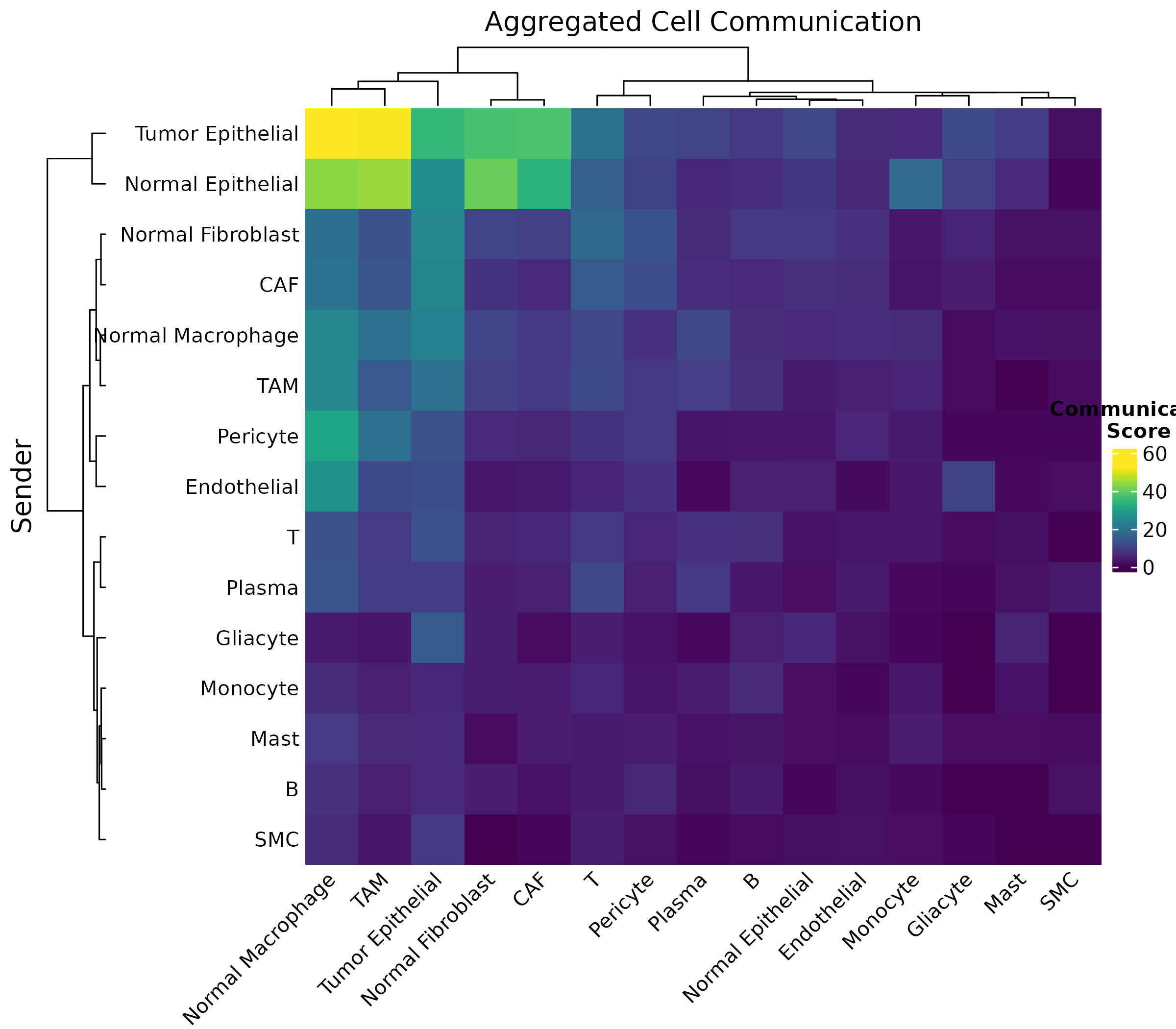
Figure 1: Communication Heatmap. Each cell shows the total communication score from sender (rows) to receiver (columns) cell types. Darker colors indicate stronger communication.
Chord Diagram
The chord diagram provides an intuitive view of communication flow between cell types.
plotCommunicationCircle(obj, top_n = 50)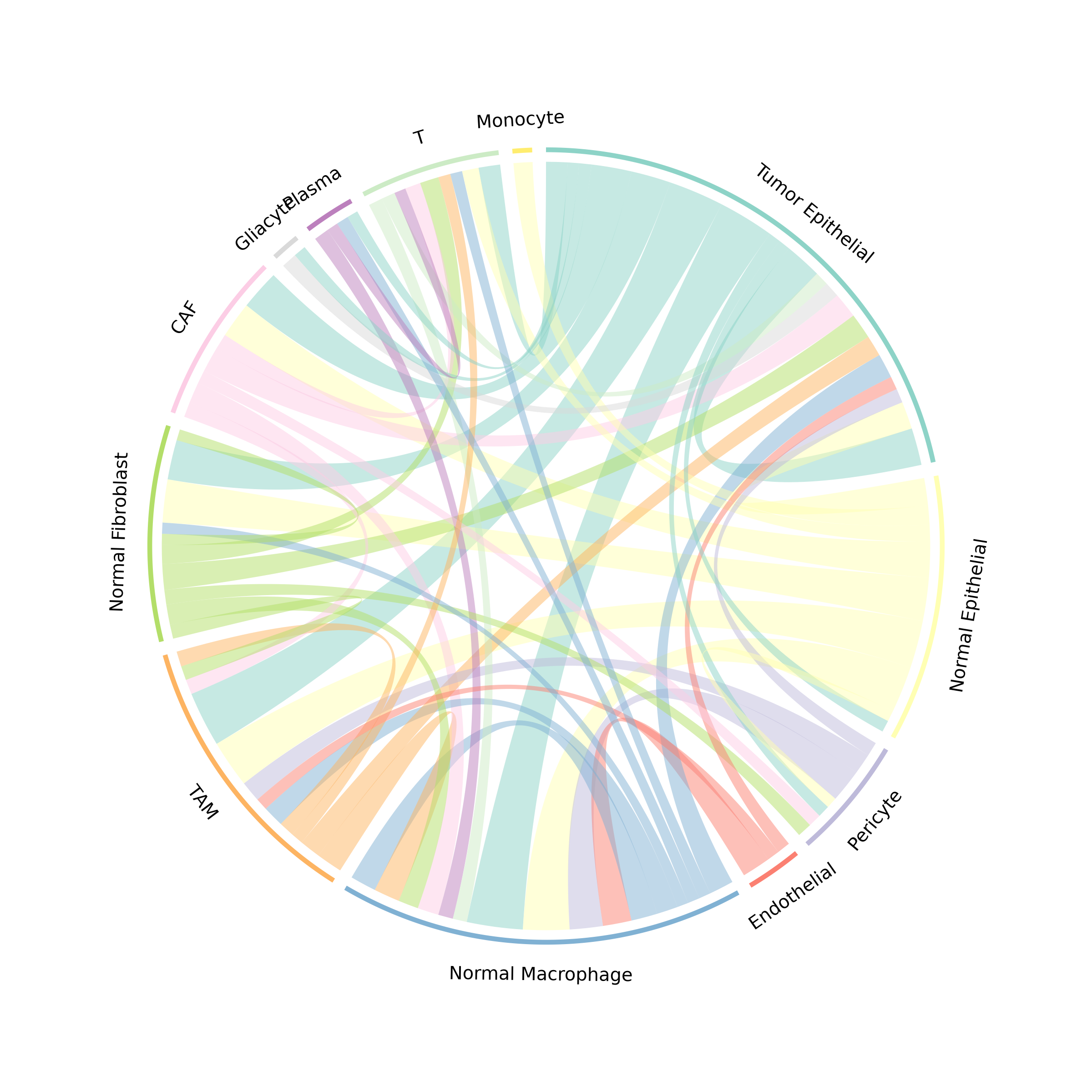
Figure 2: Communication Chord Diagram. Ribbons connect sender to receiver cell types, with width proportional to communication strength. Colors represent sender cell types.
One-Line Workflow
For convenience, you can run the entire analysis with a single function:
# Complete analysis in one line
obj <- runScMetaLink(
  expression_data = crc_expr,
  cell_meta = crc_meta,
  cell_type_column = "cell_type",
  n_permutations = 100
)
Understanding the Output
Key Objects in the Result
| Slot | Description |
|---|---|
@production_scores |
Matrix: metabolites x cell types, production potential |
@sensing_scores |
Matrix: metabolites x cell types, sensing capability |
@communication_scores |
3D array: sender x receiver x metabolite |
@communication_pvalues |
3D array: permutation p-values |
@significant_interactions |
data.frame: filtered significant interactions |
Accessing Results
# Production scores (first 5 metabolites, first 5 cell types)
obj@production_scores[1:5, 1:5]
#>             Normal Epithelial         T    Plasma Normal Fibroblast       CAF
#> HMDB0000008         0.3844017 0.3124838 0.4670759         0.3124838 0.3124838
#> HMDB0000010         0.2708579 0.2465175 0.2391890         0.5269140 0.5625056
#> HMDB0000011         0.2804398 0.3580385 0.3628140         0.5658166 0.4273138
#> HMDB0000012         0.4768788 0.4473201 0.4021738         0.3852586 0.4177708
#> HMDB0000014         0.3271932 0.4098426 0.4522973         0.3559737 0.3869064

# Significant interactions summary
cat("Total significant interactions:", nrow(obj@significant_interactions), "\n")
#> Total significant interactions: 2754
cat("\nTop metabolites involved:\n")
#>
#> Top metabolites involved:
print(head(sort(table(obj@significant_interactions$metabolite_name), decreasing = TRUE), 10))
#>
#> 11beta-Hydroxyprogesterone           5-Androstenediol
#>                         30                         23
#>                  Ornithine   7beta-Hydroxycholesterol
#>                         21                         20
#>    Adenosine monophosphate                  Cortisone
#>                         19                         19
#>                  Hydroxide                    Retinal
#>                         19                         18
#>                   L-Fucose     Uridine 5'-diphosphate
#>                         17                         17
Export Results
# Export all results to files
exportResults(obj, output_dir = "scMetaLink_results")
Next Steps
- Theory & Methods: Understand the mathematical framework
- Production & Sensing: Deep dive into inference
- Communication Analysis: Advanced communication analysis
- Spatial Analysis: Spatial transcriptomics support
- Visualization: Complete visualization guide
- Applications: Real-world analysis examples
Session Info
sessionInfo()
#> R version 4.5.2 (2025-10-31)
#> Platform: x86_64-pc-linux-gnu
#> Running under: Ubuntu 24.04.3 LTS
#>
#> Matrix products: default
#> BLAS:   /usr/lib/x86_64-linux-gnu/openblas-pthread/libblas.so.3
#> LAPACK: /usr/lib/x86_64-linux-gnu/openblas-pthread/libopenblasp-r0.3.26.so;  LAPACK version 3.12.0
#>
#> locale:
#>  [1] LC_CTYPE=C.UTF-8       LC_NUMERIC=C           LC_TIME=C.UTF-8
#>  [4] LC_COLLATE=C.UTF-8     LC_MONETARY=C.UTF-8    LC_MESSAGES=C.UTF-8
#>  [7] LC_PAPER=C.UTF-8       LC_NAME=C              LC_ADDRESS=C
#> [10] LC_TELEPHONE=C         LC_MEASUREMENT=C.UTF-8 LC_IDENTIFICATION=C
#>
#> time zone: UTC
#> tzcode source: system (glibc)
#>
#> attached base packages:
#> [1] stats     graphics  grDevices utils     datasets  methods   base
#>
#> other attached packages:
#> [1] Matrix_1.7-4      scMetaLink_0.99.1
#>
#> loaded via a namespace (and not attached):
#>  [1] viridis_0.6.5         sass_0.4.10           generics_0.1.4
#>  [4] shape_1.4.6.1         lattice_0.22-7        digest_0.6.39
#>  [7] magrittr_2.0.4        evaluate_1.0.5        grid_4.5.2
#> [10] RColorBrewer_1.1-3    iterators_1.0.14      circlize_0.4.17
#> [13] fastmap_1.2.0         foreach_1.5.2         doParallel_1.0.17
#> [16] jsonlite_2.0.0        GlobalOptions_0.1.3   gridExtra_2.3
#> [19] ComplexHeatmap_2.26.0 viridisLite_0.4.2     scales_1.4.0
#> [22] codetools_0.2-20      textshaping_1.0.4     jquerylib_0.1.4
#> [25] cli_3.6.5             rlang_1.1.7           crayon_1.5.3
#> [28] cachem_1.1.0          yaml_2.3.12           otel_0.2.0
#> [31] tools_4.5.2           parallel_4.5.2        dplyr_1.1.4
#> [34] colorspace_2.1-2      ggplot2_4.0.1         BiocGenerics_0.56.0
#> [37] GetoptLong_1.1.0      vctrs_0.7.1           R6_2.6.1
#> [40] png_0.1-8             stats4_4.5.2          matrixStats_1.5.0
#> [43] lifecycle_1.0.5       S4Vectors_0.48.0      IRanges_2.44.0
#> [46] fs_1.6.6              htmlwidgets_1.6.4     clue_0.3-66
#> [49] cluster_2.1.8.1       ragg_1.5.0            pkgconfig_2.0.3
#> [52] desc_1.4.3            pkgdown_2.2.0         pillar_1.11.1
#> [55] bslib_0.9.0           gtable_0.3.6          glue_1.8.0
#> [58] systemfonts_1.3.1     xfun_0.56             tibble_3.3.1
#> [61] tidyselect_1.2.1      knitr_1.51            farver_2.1.2
#> [64] rjson_0.2.23          htmltools_0.5.9       rmarkdown_2.30
#> [67] compiler_4.5.2        S7_0.2.1