Advanced Usage

Introduction

This vignette covers advanced features of darwin for power users, including custom objective functions, fixed gene count mode, parallel computing, and integration with other tools.

library(darwin)
library(ggplot2)
set.seed(42)

Prepare Data

# Create reference matrix
n_ct <- 5
n_genes <- 400
reference <- matrix(abs(rnorm(n_ct * n_genes, 2, 1)), nrow = n_ct, ncol = n_genes)
rownames(reference) <- paste0("CellType", 1:n_ct)
colnames(reference) <- paste0("Gene", 1:n_genes)

# Add markers
for (i in 1:n_ct) {
  reference[i, ((i-1)*20+1):(i*20)] <- reference[i, ((i-1)*20+1):(i*20)] + 4
}

Custom Objective Functions

darwin allows you to define custom objective functions for specialized applications.

Requirements

A valid objective function must:

Accept a single argument: data matrix (cell types × genes)
Return a single numeric value
Be consistent (same input → same output)

Example: Variance Objective

# Custom objective: maximize total variance
variance_objective <- function(data) {
  sum(apply(data, 2, var))
}

# Test the function
test_data <- reference[, 1:50]
cat("Variance objective value:", variance_objective(test_data), "\n")
#> Variance objective value: 200.312

Example: Marker Score Objective

# Custom objective: maximize marker specificity
# Higher when genes are specific to individual cell types
marker_score <- function(data) {
  # Max expression / mean expression ratio
  col_max <- apply(data, 2, max)
  col_mean <- colMeans(data)
  col_mean[col_mean == 0] <- 1e-10
  sum(col_max / col_mean)
}

cat("Marker score value:", marker_score(test_data), "\n")
#> Marker score value: 107.8375

Using Custom Objectives

dw_custom <- darwin(reference)
dw_custom$optimize(
  ngen = 60,
  objectives = c("correlation", variance_objective),
  weights = c(-1, 1),  # Minimize correlation, maximize variance
  verbose = FALSE,
  parallel = FALSE
)

# The second objective column will show variance values
fitness <- dw_custom$get_fitness()
colnames(fitness) <- c("Correlation", "Variance")

ggplot(as.data.frame(fitness), aes(x = Correlation, y = Variance)) +
  geom_point(color = "#3498db", size = 3, alpha = 0.7) +
  geom_line(color = "gray60", alpha = 0.5) +
  labs(
    title = "Custom Objectives: Correlation vs Variance",
    subtitle = "Minimize correlation, maximize variance",
    x = "Correlation (lower is better)",
    y = "Variance (higher is better)"
  ) +
  theme_minimal(base_size = 12)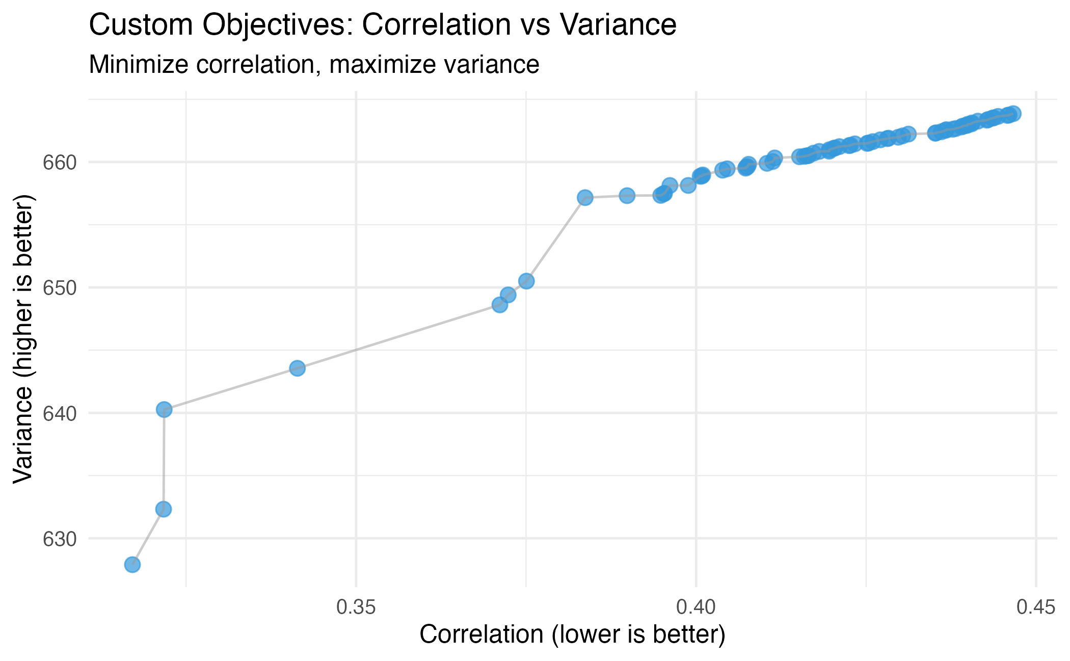

Pareto front with custom objectives: correlation vs variance.

Three Objectives

dw_three <- darwin(reference)
dw_three$optimize(
  ngen = 60,
  objectives = c("correlation", "distance", "condition"),
  weights = c(-1, 1, -1),  # Minimize corr/cond, maximize distance
  verbose = FALSE,
  parallel = FALSE
)

fitness3 <- dw_three$get_fitness()
cat("Three-objective optimization:\n")
#> Three-objective optimization:
cat("  Solutions:", nrow(fitness3), "\n")
#>   Solutions: 314
cat("  Correlation range:", round(range(fitness3[,1]), 2), "\n")
#>   Correlation range: 0.21 0.79
cat("  Distance range:", round(range(fitness3[,2]), 2), "\n")
#>   Distance range: 143.43 363.86
cat("  Condition range:", round(range(fitness3[,3]), 2), "\n")
#>   Condition range: 3.93 4.27

Fixed Gene Count Mode

For applications requiring a specific number of marker genes, use fixed mode:

dw_fixed <- darwin(reference)
dw_fixed$optimize(
  ngen = 60,
  mode = "fixed",
  n_features = 50,  # Select exactly 50 genes
  objectives = c("correlation", "distance"),
  weights = c(-1, 1),
  verbose = FALSE,
  parallel = FALSE
)

# Verify all solutions have 50 genes
pareto <- dw_fixed$get_pareto()
gene_counts <- sapply(pareto, sum)
cat("Gene counts in fixed mode:", unique(gene_counts), "\n")
#> Gene counts in fixed mode: 50

# Compare gene count distributions
df_compare <- rbind(
  data.frame(
    mode = "Standard",
    n_genes = sapply(dw_custom$get_pareto(), sum)
  ),
  data.frame(
    mode = "Fixed (50)",
    n_genes = gene_counts
  )
)

ggplot(df_compare, aes(x = n_genes, fill = mode)) +
  geom_histogram(bins = 20, alpha = 0.7, position = "identity") +
  scale_fill_manual(values = c("#3498db", "#e74c3c")) +
  labs(
    title = "Gene Count Distribution: Standard vs Fixed Mode",
    x = "Number of Selected Genes",
    y = "Frequency"
  ) +
  theme_minimal(base_size = 12)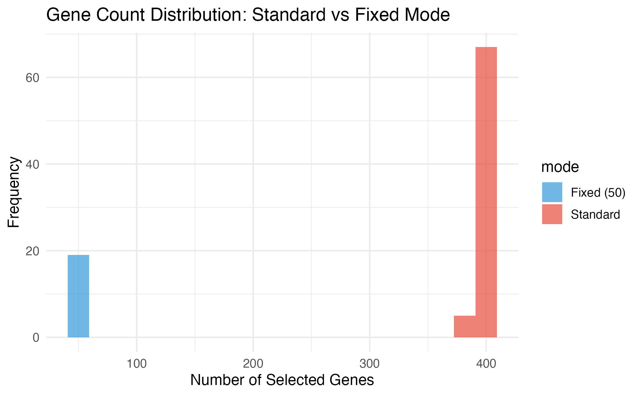

Fixed mode ensures all solutions have exactly the specified number of genes.

Selection Strategies

darwin provides flexible selection from the Pareto front:

1. Weighted Selection

dw <- darwin(reference)
dw$optimize(ngen = 50, verbose = FALSE, parallel = FALSE)

# Emphasize minimizing correlation
dw$select(weights = c(-2, 1))
cat("Emphasize correlation - genes:", sum(dw$get_selection()), "\n")
#> Emphasize correlation - genes: 388

# Emphasize maximizing distance
dw$select(weights = c(-1, 2))
cat("Emphasize distance - genes:", sum(dw$get_selection()), "\n")
#> Emphasize distance - genes: 388

2. Index-Based Selection

# Select by direct index
dw$select(index = 1)
cat("Solution 1 - genes:", sum(dw$get_selection()), "\n")
#> Solution 1 - genes: 400

# Select by objective rank
# (objective_index, rank) - rank 1 = best for that objective
dw$select(index = c(1, 1))  # Best correlation
cat("Best correlation - genes:", sum(dw$get_selection()), "\n")
#> Best correlation - genes: 326

dw$select(index = c(2, -1))  # Best distance (last rank)
cat("Best distance - genes:", sum(dw$get_selection()), "\n")
#> Best distance - genes: 400

3. Target Value Selection

# Select solution closest to target correlation value
fitness <- dw$get_fitness()
target_corr <- median(fitness$correlation)
dw$select(close_to = c(1, target_corr))
cat("Target correlation", round(target_corr, 2), "- genes:", sum(dw$get_selection()), "\n")
#> Target correlation 0.42 - genes: 397

Parallel Computing

darwin supports parallel computation for faster optimization:

# Enable parallel computing
options(darwin.parallel = TRUE)

# Or specify in optimize()
dw$optimize(
  ngen = 100,
  parallel = TRUE,  # Uses all available cores - 1
  verbose = TRUE
)

# Disable parallel computing
options(darwin.parallel = FALSE)

Performance Comparison

# Benchmark (example, not run)
library(microbenchmark)

# Large dataset
large_ref <- matrix(rnorm(50 * 2000), nrow = 50)

microbenchmark(
  serial = {
    dw <- darwin(large_ref)
    dw$optimize(ngen = 10, parallel = FALSE, verbose = FALSE)
  },
  parallel = {
    dw <- darwin(large_ref)
    dw$optimize(ngen = 10, parallel = TRUE, verbose = FALSE)
  },
  times = 3
)

Parameter Tuning

Population Size

Larger populations provide more diversity but slower convergence:

results <- list()
for (pop in c(30, 60, 100)) {
  dw_temp <- darwin(reference)
  dw_temp$optimize(
    ngen = 40,
    pop_size = pop,
    verbose = FALSE,
    parallel = FALSE
  )
  results[[as.character(pop)]] <- data.frame(
    dw_temp$get_fitness(),
    pop_size = factor(pop)
  )
}

df_pop <- do.call(rbind, results)

ggplot(df_pop, aes(x = correlation, y = distance, color = pop_size)) +
  geom_point(alpha = 0.6) +
  scale_color_brewer(palette = "Set1") +
  labs(
    title = "Effect of Population Size",
    x = "Correlation",
    y = "Distance",
    color = "Population\nSize"
  ) +
  theme_minimal(base_size = 12)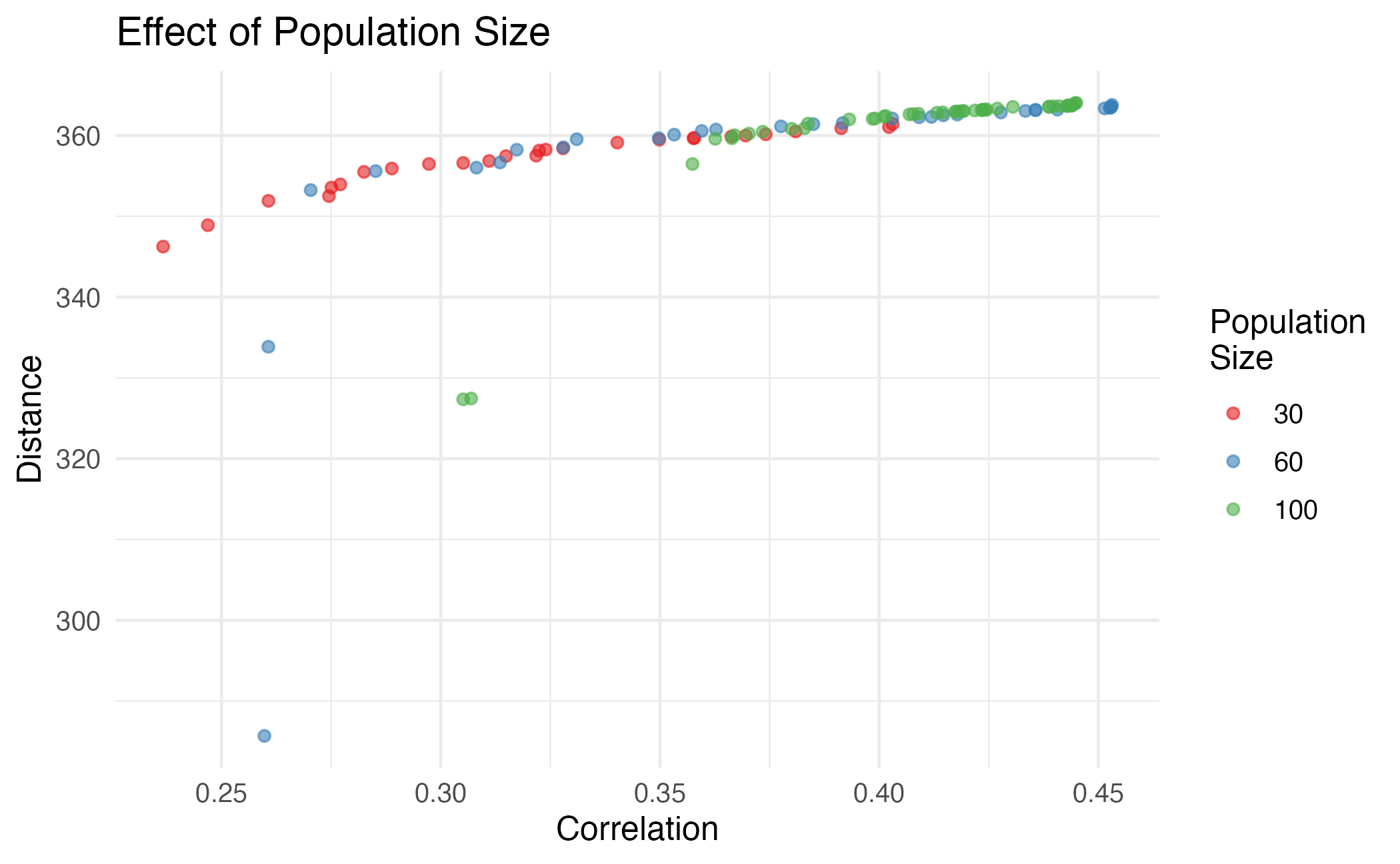

Effect of population size on Pareto front diversity.

Mutation Probability

Higher mutation enables more exploration:

results_mut <- list()
for (mut in c(0.001, 0.01, 0.05)) {
  dw_temp <- darwin(reference)
  dw_temp$optimize(
    ngen = 40,
    mutation_prob = mut,
    verbose = FALSE,
    parallel = FALSE
  )
  
  pareto <- dw_temp$get_pareto()
  gene_counts <- sapply(pareto, sum)
  
  results_mut[[as.character(mut)]] <- data.frame(
    n_genes = gene_counts,
    mutation = factor(mut)
  )
}

df_mut <- do.call(rbind, results_mut)

ggplot(df_mut, aes(x = n_genes, fill = mutation)) +
  geom_density(alpha = 0.5) +
  scale_fill_brewer(palette = "Set1") +
  labs(
    title = "Effect of Mutation Probability on Gene Count",
    x = "Number of Selected Genes",
    y = "Density",
    fill = "Mutation\nProbability"
  ) +
  theme_minimal(base_size = 12)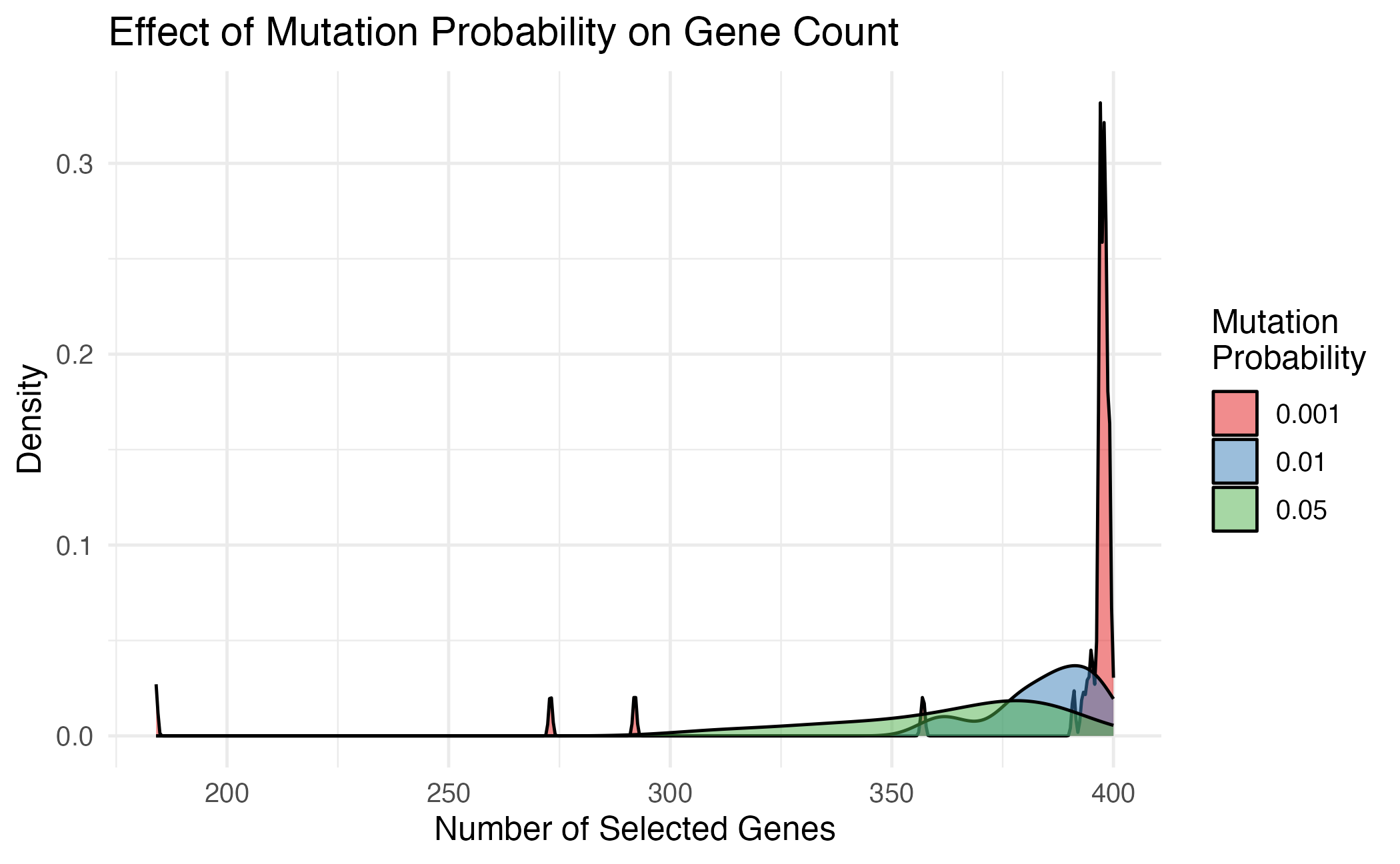

Effect of mutation probability on solution diversity.

Save and Load

darwin objects can be saved and loaded for reproducibility:

# Save
temp_file <- tempfile(fileext = ".rds")
dw$save(temp_file)

# Load
dw_loaded <- readRDS(temp_file)

# Verify
cat("Original Pareto size:", length(dw$get_pareto()), "\n")
#> Original Pareto size: 99
cat("Loaded Pareto size:", length(dw_loaded$get_pareto()), "\n")
#> Loaded Pareto size: 99

# Clean up
unlink(temp_file)

Integration Examples

With Seurat

library(Seurat)

# From Seurat object with annotations
dw <- darwin(
  seurat_obj,
  celltype_key = "cell_type",
  assay = "RNA",
  layer = "data",
  use_highly_variable = TRUE
)

# Optimize and select
dw$optimize(ngen = 100)
dw$select()

# Get marker genes
markers <- dw$get_genes()

Export to Other Deconvolution Tools

# Get selected genes for use with other tools
genes <- dw$get_genes()
selection <- dw$get_selection()

# Create signature matrix for CIBERSORT
signature_matrix <- reference[, selection]
write.csv(signature_matrix, "signature_matrix.csv")

# Or as gene list for MuSiC
gene_list <- genes

Troubleshooting

Common Issues

Slow optimization: Reduce ngen, pop_size, or enable parallel = TRUE
Poor convergence: Increase ngen or pop_size
All solutions identical: Increase mutation_prob
Memory issues: Use gene pre-selection with use_highly_variable = TRUE

Diagnostic Checks

# Check optimization quality
fitness <- dw$get_fitness()

cat("Diagnostic Summary:\n")
#> Diagnostic Summary:
cat("  Pareto front size:", nrow(fitness), "\n")
#>   Pareto front size: 99
cat("  Correlation range:", round(diff(range(fitness[,1])), 3), "\n")
#>   Correlation range: 0.149
cat("  Distance range:", round(diff(range(fitness[,2])), 3), "\n")
#>   Distance range: 47.774
cat("  Gene count range:", range(sapply(dw$get_pareto(), sum)), "\n")
#>   Gene count range: 326 400

Session Info

sessionInfo()
#> R version 4.4.0 (2024-04-24)
#> Platform: aarch64-apple-darwin20
#> Running under: macOS 15.6.1
#> 
#> Matrix products: default
#> BLAS:   /Library/Frameworks/R.framework/Versions/4.4-arm64/Resources/lib/libRblas.0.dylib 
#> LAPACK: /Library/Frameworks/R.framework/Versions/4.4-arm64/Resources/lib/libRlapack.dylib;  LAPACK version 3.12.0
#> 
#> locale:
#> [1] C
#> 
#> time zone: Asia/Shanghai
#> tzcode source: internal
#> 
#> attached base packages:
#> [1] stats     graphics  grDevices utils     datasets  methods   base     
#> 
#> other attached packages:
#> [1] ggplot2_4.0.1 darwin_1.0.0 
#> 
#> loaded via a namespace (and not attached):
#>  [1] sass_0.4.10         future_1.69.0       generics_0.1.4     
#>  [4] lattice_0.22-7      listenv_0.10.0      digest_0.6.39      
#>  [7] magrittr_2.0.4      evaluate_1.0.5      grid_4.4.0         
#> [10] RColorBrewer_1.1-3  fastmap_1.2.0       jsonlite_2.0.0     
#> [13] Matrix_1.7-4        scales_1.4.0        codetools_0.2-20   
#> [16] textshaping_1.0.4   jquerylib_0.1.4     cli_3.6.5          
#> [19] rlang_1.1.7         parallelly_1.46.1   future.apply_1.20.1
#> [22] withr_3.0.2         cachem_1.1.0        yaml_2.3.12        
#> [25] otel_0.2.0          tools_4.4.0         parallel_4.4.0     
#> [28] dplyr_1.1.4         globals_0.18.0      vctrs_0.7.1        
#> [31] R6_2.6.1            lifecycle_1.0.5     fs_1.6.6           
#> [34] htmlwidgets_1.6.4   ragg_1.5.0          pkgconfig_2.0.3    
#> [37] desc_1.4.3          pkgdown_2.1.3       pillar_1.11.1      
#> [40] bslib_0.9.0         gtable_0.3.6        glue_1.8.0         
#> [43] Rcpp_1.1.1          systemfonts_1.3.1   xfun_0.56          
#> [46] tibble_3.3.1        tidyselect_1.2.1    knitr_1.51         
#> [49] dichromat_2.0-0.1   farver_2.1.2        htmltools_0.5.9    
#> [52] rmarkdown_2.30      labeling_0.4.3      compiler_4.4.0     
#> [55] S7_0.2.1

Zaoqu Liu

2026-01-25