Introduction
This vignette demonstrates darwin’s performance characteristics and provides benchmarks for different problem sizes and configurations. Understanding these benchmarks helps users make informed decisions about parameter settings for their specific use cases.
Performance Architecture
darwin achieves high performance through several design choices:
- Vectorized R operations for matrix computations
- C++ implementations (via RcppArmadillo) for critical operations
-
Parallel processing support via the
futurepackage - Efficient memory management using sparse representations where appropriate
C++ vs R Performance
# Create test data
n_ct <- 10
n_genes <- 100
test_data <- matrix(runif(n_ct * n_genes), nrow = n_ct)

# Compare implementations
n_iter <- 50
times_r <- numeric(n_iter)
times_cpp <- numeric(n_iter)

for (i in 1:n_iter) {
  t1 <- system.time({
    compute_correlation(test_data, use_cpp = FALSE)
  })
  times_r[i] <- t1["elapsed"]

  t2 <- system.time({
    compute_correlation(test_data, use_cpp = TRUE)
  })
  times_cpp[i] <- t2["elapsed"]
}

df_bench <- data.frame(
  Time = c(times_r, times_cpp) * 1000,
  Implementation = rep(c("R (vectorized)", "C++ (RcppArmadillo)"), each = n_iter)
)

ggplot(df_bench, aes(x = Implementation, y = Time, fill = Implementation)) +
  geom_boxplot(alpha = 0.7) +
  scale_fill_manual(values = c("#e74c3c", "#3498db")) +
  labs(
    title = "R vs C++ Implementation Performance",
    subtitle = paste("Computing correlation for", n_ct, "× ", n_genes, "matrix"),
    x = "",
    y = "Time (milliseconds)"
  ) +
  theme_minimal(base_size = 12) +
  theme(legend.position = "none")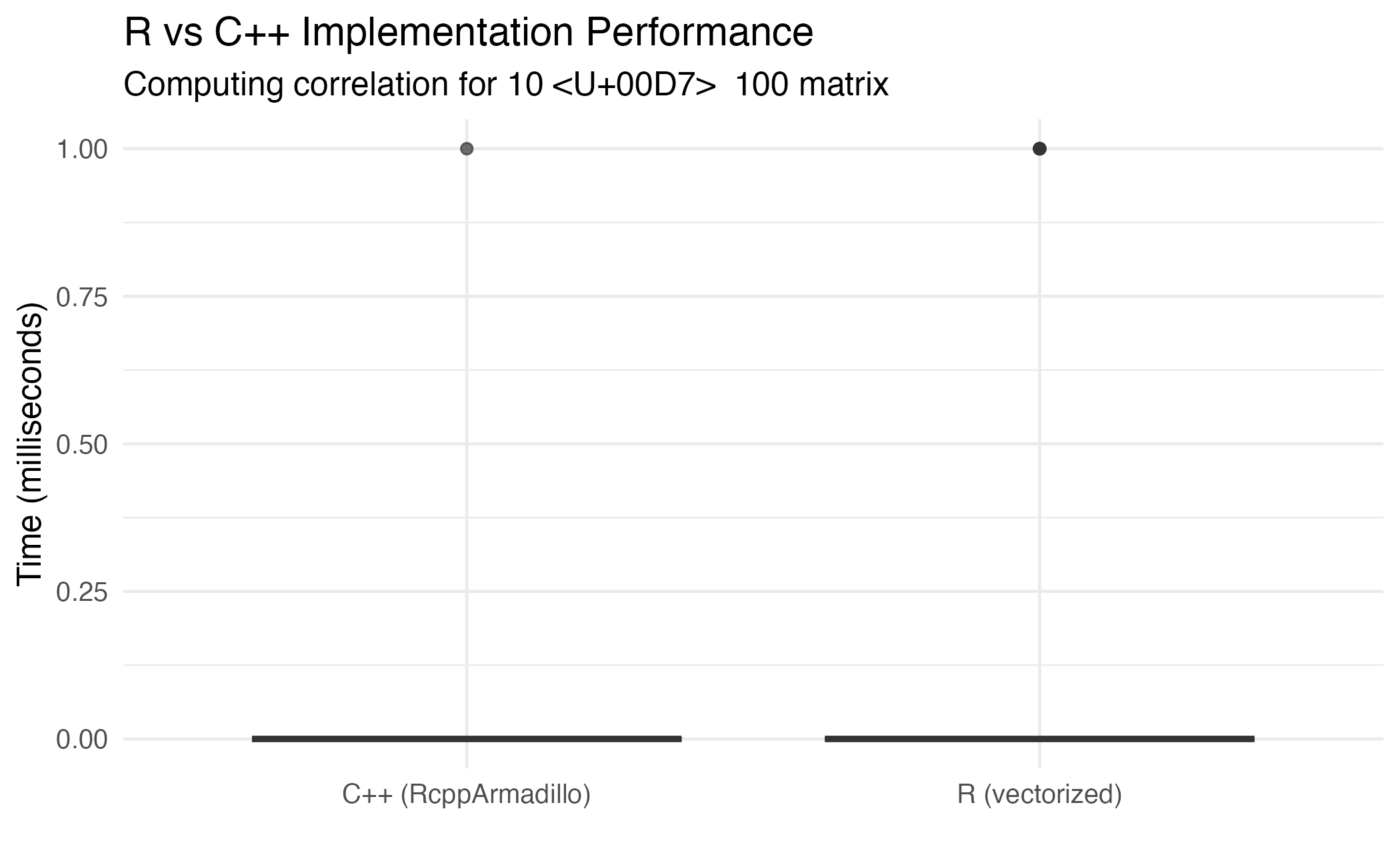
Performance comparison between R and C++ implementations.
Scaling with Problem Size
Number of Genes
gene_sizes <- c(100, 200, 500, 1000, 2000)
n_ct <- 8
results <- list()

for (n_genes in gene_sizes) {
  test_data <- matrix(runif(n_ct * n_genes), nrow = n_ct)

  # Time correlation computation
  t <- system.time({
    for (j in 1:20) {
      compute_correlation(test_data, use_cpp = TRUE)
    }
  })

  results[[length(results) + 1]] <- data.frame(
    n_genes = n_genes,
    time = t["elapsed"] / 20 * 1000
  )
}

df_scale_genes <- do.call(rbind, results)

ggplot(df_scale_genes, aes(x = n_genes, y = time)) +
  geom_line(color = "#3498db", linewidth = 1) +
  geom_point(color = "#3498db", size = 3) +
  scale_x_log10() +
  scale_y_log10() +
  labs(
    title = "Performance Scaling with Gene Count",
    subtitle = paste(n_ct, "cell types"),
    x = "Number of Genes (log scale)",
    y = "Time per iteration (ms, log scale)"
  ) +
  theme_minimal(base_size = 12)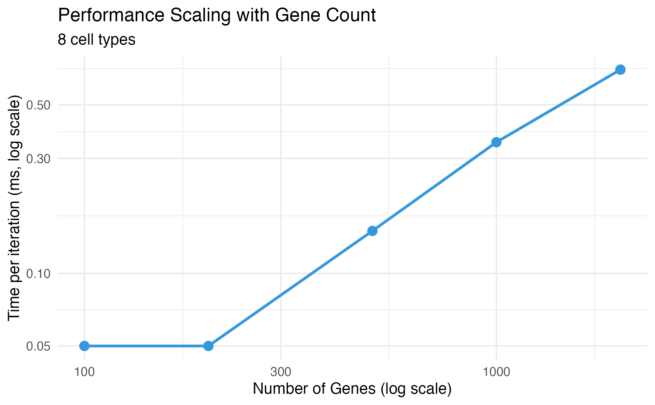
Performance scaling with number of genes.
Number of Cell Types
ct_sizes <- c(3, 5, 10, 20, 30)
n_genes <- 500
results_ct <- list()

for (n_ct in ct_sizes) {
  test_data <- matrix(runif(n_ct * n_genes), nrow = n_ct)

  t <- system.time({
    for (j in 1:20) {
      compute_correlation(test_data, use_cpp = TRUE)
    }
  })

  results_ct[[length(results_ct) + 1]] <- data.frame(
    n_ct = n_ct,
    time = t["elapsed"] / 20 * 1000
  )
}

df_scale_ct <- do.call(rbind, results_ct)

ggplot(df_scale_ct, aes(x = n_ct, y = time)) +
  geom_line(color = "#e74c3c", linewidth = 1) +
  geom_point(color = "#e74c3c", size = 3) +
  labs(
    title = "Performance Scaling with Cell Type Count",
    subtitle = paste(n_genes, "genes"),
    x = "Number of Cell Types",
    y = "Time per iteration (ms)"
  ) +
  theme_minimal(base_size = 12)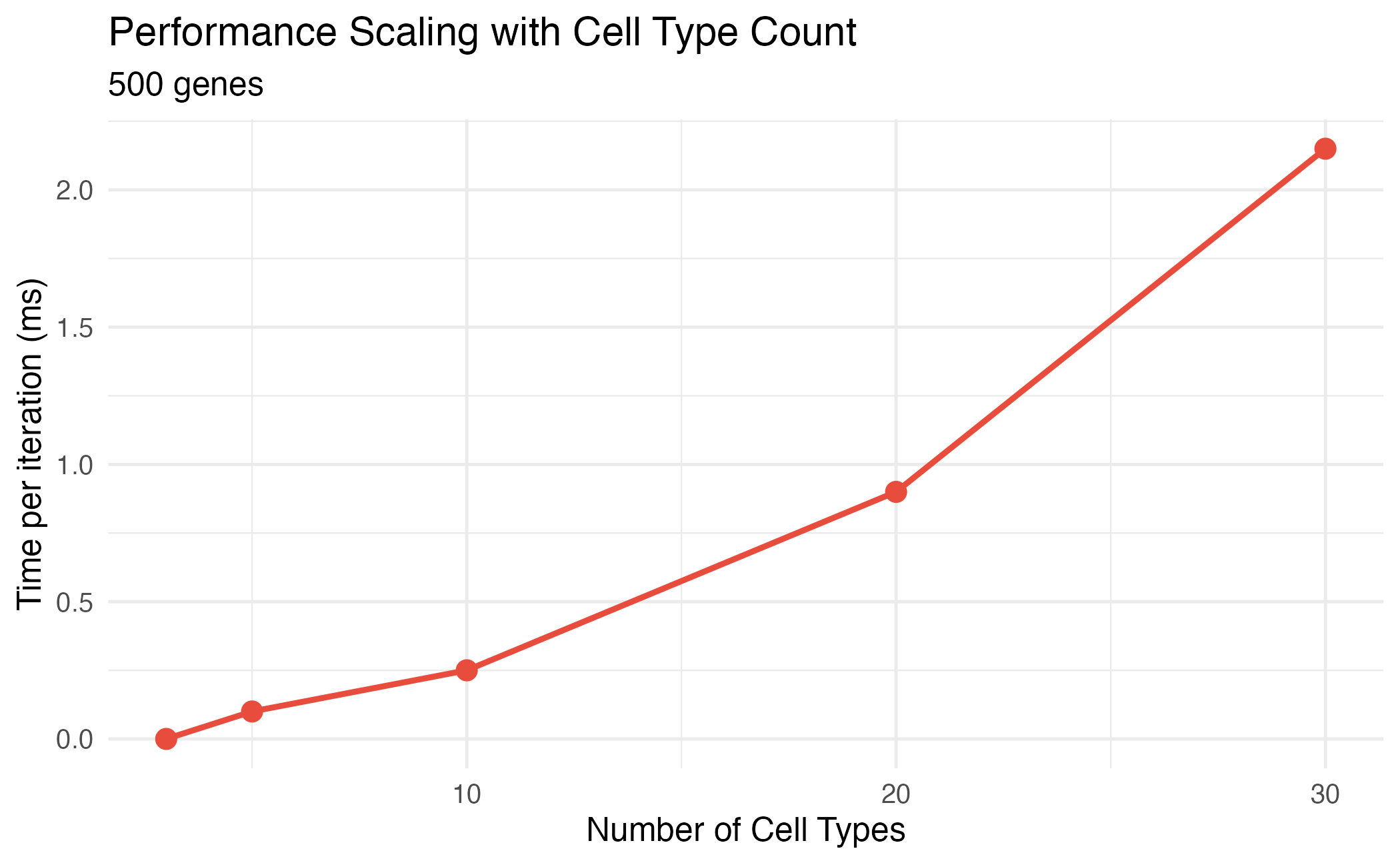
Performance scaling with number of cell types.
Optimization Benchmarks
Complete Workflow Timing
# Setup
n_ct <- 8
n_genes <- 1000
reference <- matrix(abs(rnorm(n_ct * n_genes, 2)), nrow = n_ct)
rownames(reference) <- paste0("CT", 1:n_ct)
colnames(reference) <- paste0("Gene", 1:n_genes)

# Benchmark components
timings <- list()

# Initialization
t_init <- system.time({
  dw <- darwin(reference)
})
timings$Initialization <- t_init["elapsed"]

# Optimization (short run for benchmark)
t_opt <- system.time({
  dw$optimize(ngen = 20, pop_size = 50, verbose = FALSE, parallel = FALSE)
})
timings$Optimization <- t_opt["elapsed"]

# Selection
t_sel <- system.time({
  dw$select(weights = c(-1, 1))
})
timings$Selection <- t_sel["elapsed"]

# Create timing data frame
df_timing <- data.frame(
  Step = names(timings),
  Time = unlist(timings)
)
df_timing$Percent <- df_timing$Time / sum(df_timing$Time) * 100

ggplot(df_timing, aes(x = reorder(Step, Time), y = Time, fill = Step)) +
  geom_bar(stat = "identity", alpha = 0.8) +
  geom_text(aes(label = paste0(round(Percent, 1), "%")), hjust = -0.1) +
  coord_flip() +
  scale_fill_brewer(palette = "Set2") +
  labs(
    title = "Workflow Time Breakdown",
    subtitle = paste(n_genes, "genes,", n_ct, "cell types, 20 generations"),
    x = "",
    y = "Time (seconds)"
  ) +
  theme_minimal(base_size = 12) +
  theme(legend.position = "none") +
  expand_limits(y = max(df_timing$Time) * 1.2)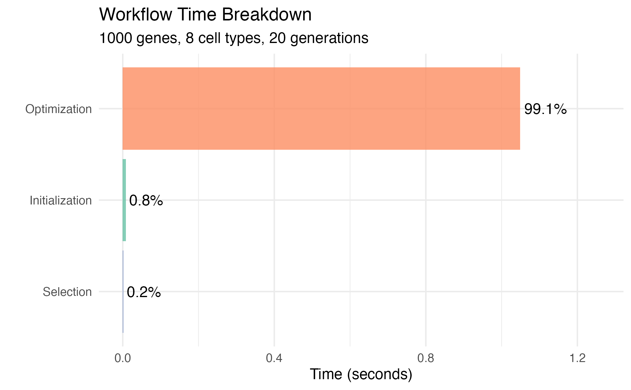
Time breakdown for a complete optimization workflow.
Scaling with Generations
gen_sizes <- c(10, 25, 50, 100)
results_gen <- list()

for (ngen in gen_sizes) {
  t <- system.time({
    dw <- darwin(reference)
    dw$optimize(ngen = ngen, pop_size = 50, verbose = FALSE, parallel = FALSE)
  })

  results_gen[[length(results_gen) + 1]] <- data.frame(
    generations = ngen,
    time = t["elapsed"]
  )
}

df_scale_gen <- do.call(rbind, results_gen)

# Fit linear model
lm_fit <- lm(time ~ generations, data = df_scale_gen)

ggplot(df_scale_gen, aes(x = generations, y = time)) +
  geom_line(color = "#3498db", linewidth = 1) +
  geom_point(color = "#3498db", size = 3) +
  geom_smooth(method = "lm", se = FALSE, linetype = "dashed", color = "gray50") +
  labs(
    title = "Scaling with Number of Generations",
    subtitle = paste("~", round(coef(lm_fit)[2], 3), "seconds per generation"),
    x = "Number of Generations",
    y = "Total Time (seconds)"
  ) +
  theme_minimal(base_size = 12)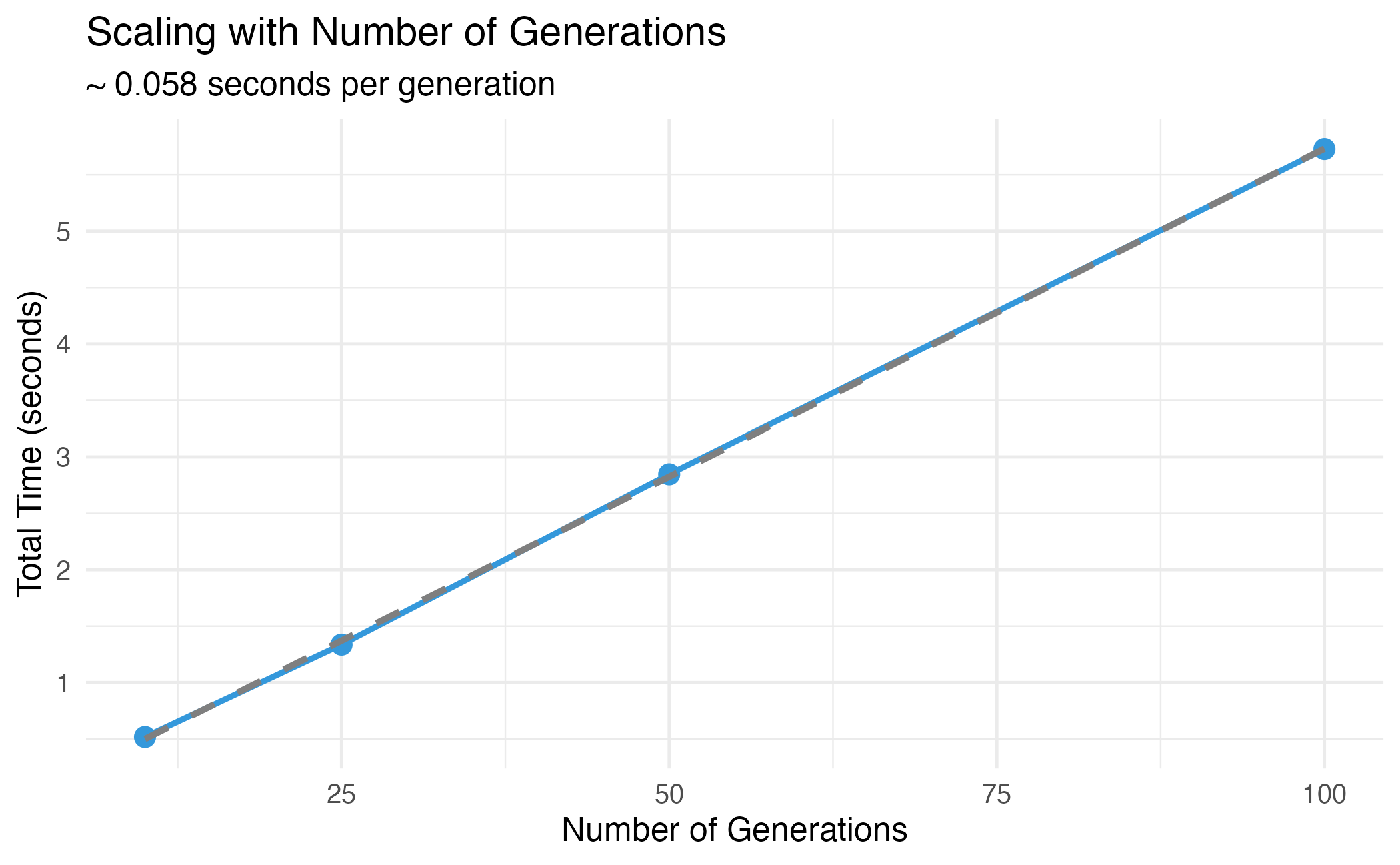
Linear scaling with number of generations.
Scaling with Population Size
pop_sizes <- c(30, 50, 80, 100, 150)
results_pop <- list()

for (pop in pop_sizes) {
  t <- system.time({
    dw <- darwin(reference)
    dw$optimize(ngen = 30, pop_size = pop, verbose = FALSE, parallel = FALSE)
  })

  results_pop[[length(results_pop) + 1]] <- data.frame(
    pop_size = pop,
    time = t["elapsed"]
  )
}

df_scale_pop <- do.call(rbind, results_pop)

ggplot(df_scale_pop, aes(x = pop_size, y = time)) +
  geom_line(color = "#e74c3c", linewidth = 1) +
  geom_point(color = "#e74c3c", size = 3) +
  labs(
    title = "Scaling with Population Size",
    subtitle = "30 generations",
    x = "Population Size",
    y = "Total Time (seconds)"
  ) +
  theme_minimal(base_size = 12)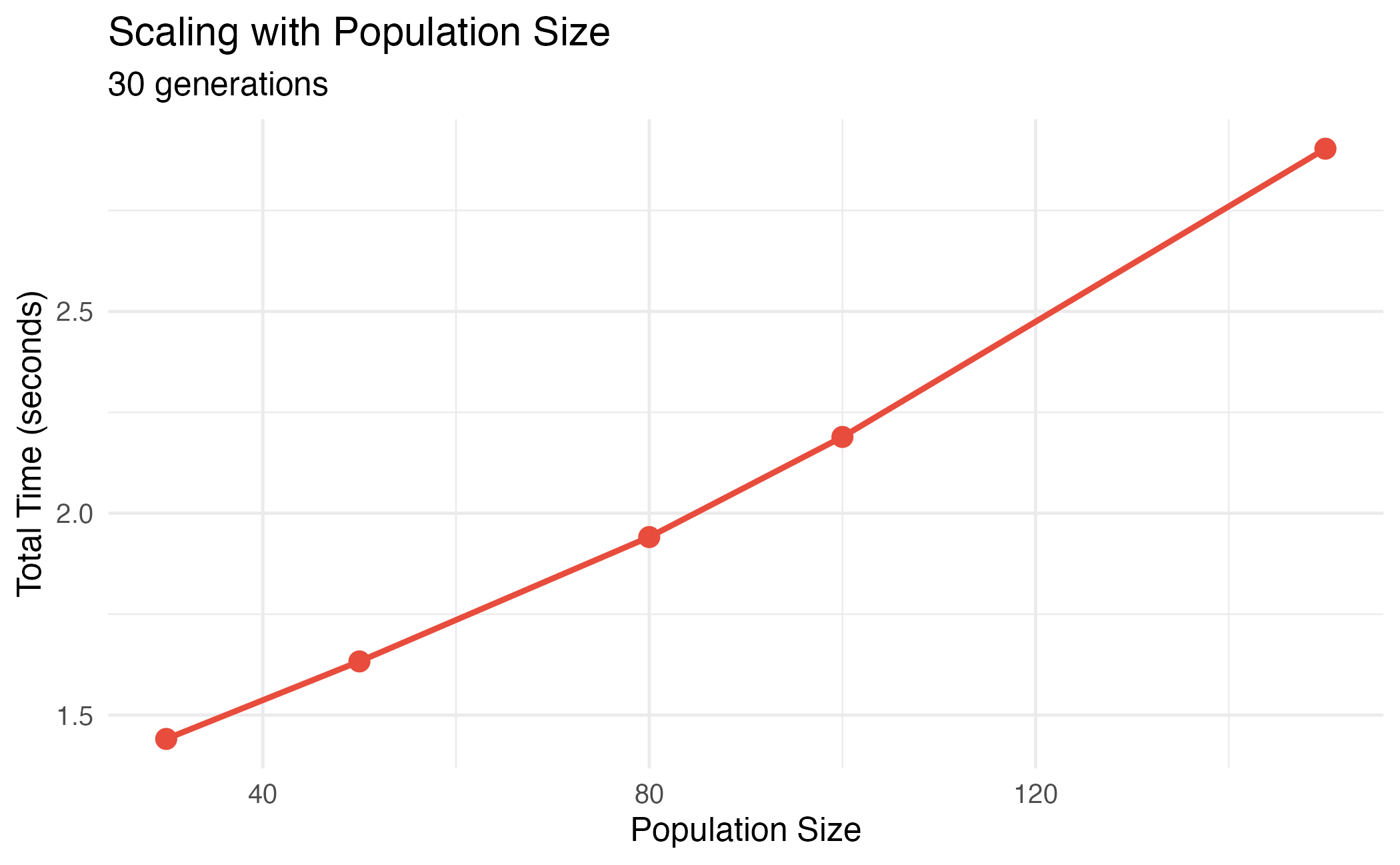
Performance scaling with population size.
Objective Function Comparison
test_data <- matrix(runif(10 * 500), nrow = 10)
n_iter <- 100

obj_times <- data.frame(
  Objective = character(),
  Time = numeric(),
  stringsAsFactors = FALSE
)

# Correlation
t <- system.time({
  for (i in 1:n_iter) compute_correlation(test_data, use_cpp = TRUE)
})
obj_times <- rbind(obj_times, data.frame(Objective = "Correlation", Time = t["elapsed"] / n_iter * 1000))

# Distance
t <- system.time({
  for (i in 1:n_iter) compute_distance(test_data, use_cpp = TRUE)
})
obj_times <- rbind(obj_times, data.frame(Objective = "Distance", Time = t["elapsed"] / n_iter * 1000))

# Condition
t <- system.time({
  for (i in 1:n_iter) compute_condition(test_data, use_cpp = TRUE)
})
obj_times <- rbind(obj_times, data.frame(Objective = "Condition", Time = t["elapsed"] / n_iter * 1000))

ggplot(obj_times, aes(x = reorder(Objective, Time), y = Time, fill = Objective)) +
  geom_bar(stat = "identity", alpha = 0.8) +
  coord_flip() +
  scale_fill_brewer(palette = "Set2") +
  labs(
    title = "Objective Function Computation Time",
    subtitle = "10 cell types × 500 genes, C++ implementation",
    x = "",
    y = "Time per call (ms)"
  ) +
  theme_minimal(base_size = 12) +
  theme(legend.position = "none")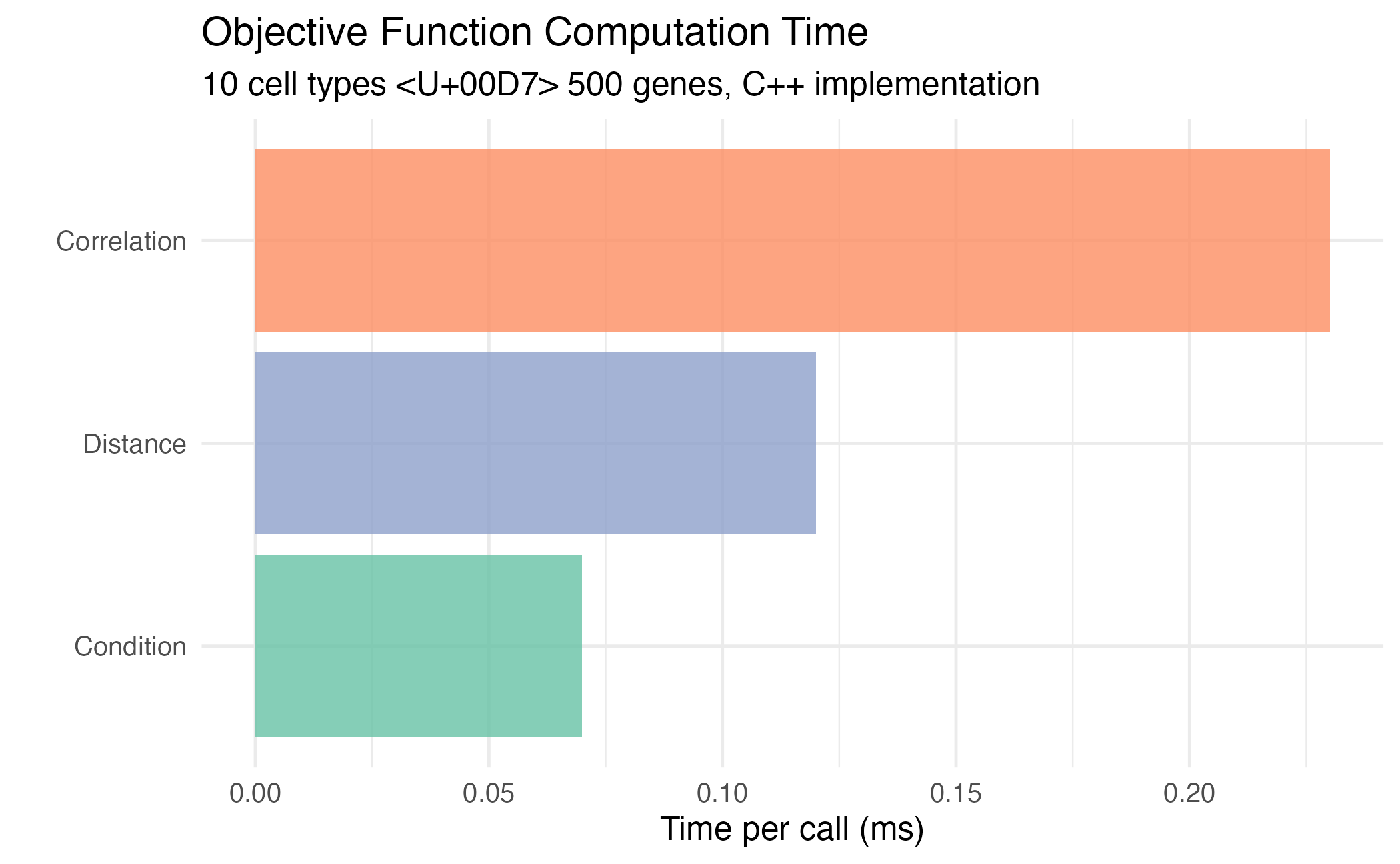
Comparison of objective function computation times.
Memory Usage
darwin is designed to be memory-efficient:
# Memory usage estimation (not run in vignette)
library(pryr)

# Reference data
n_ct <- 10
n_genes <- 5000
reference <- matrix(rnorm(n_ct * n_genes), nrow = n_ct)

# Memory for reference
cat("Reference matrix:", object_size(reference) / 1e6, "MB\n")

# Memory for darwin object
dw <- darwin(reference)
cat("darwin object (initialized):", object_size(dw) / 1e6, "MB\n")

# After optimization
dw$optimize(ngen = 50, verbose = FALSE)
cat("darwin object (optimized):", object_size(dw) / 1e6, "MB\n")
Recommendations
Based on these benchmarks:
| Problem Size | Recommended Settings |
|---|---|
| Small (<500 genes) |
ngen = 100, pop_size = 100
|
| Medium (500-2000 genes) |
ngen = 80, pop_size = 80
|
| Large (>2000 genes) |
ngen = 50, pop_size = 50, enable
parallel |
Session Info
sessionInfo()
#> R version 4.4.0 (2024-04-24)
#> Platform: aarch64-apple-darwin20
#> Running under: macOS 15.6.1
#>
#> Matrix products: default
#> BLAS:   /Library/Frameworks/R.framework/Versions/4.4-arm64/Resources/lib/libRblas.0.dylib
#> LAPACK: /Library/Frameworks/R.framework/Versions/4.4-arm64/Resources/lib/libRlapack.dylib;  LAPACK version 3.12.0
#>
#> locale:
#> [1] C
#>
#> time zone: Asia/Shanghai
#> tzcode source: internal
#>
#> attached base packages:
#> [1] stats     graphics  grDevices utils     datasets  methods   base
#>
#> other attached packages:
#> [1] ggplot2_4.0.1 darwin_1.0.0
#>
#> loaded via a namespace (and not attached):
#>  [1] sass_0.4.10         future_1.69.0       generics_0.1.4
#>  [4] lattice_0.22-7      listenv_0.10.0      digest_0.6.39
#>  [7] magrittr_2.0.4      evaluate_1.0.5      grid_4.4.0
#> [10] RColorBrewer_1.1-3  fastmap_1.2.0       jsonlite_2.0.0
#> [13] Matrix_1.7-4        mgcv_1.9-3          scales_1.4.0
#> [16] codetools_0.2-20    textshaping_1.0.4   jquerylib_0.1.4
#> [19] cli_3.6.5           rlang_1.1.7         parallelly_1.46.1
#> [22] future.apply_1.20.1 splines_4.4.0       withr_3.0.2
#> [25] cachem_1.1.0        yaml_2.3.12         otel_0.2.0
#> [28] tools_4.4.0         parallel_4.4.0      dplyr_1.1.4
#> [31] globals_0.18.0      vctrs_0.7.1         R6_2.6.1
#> [34] lifecycle_1.0.5     fs_1.6.6            htmlwidgets_1.6.4
#> [37] ragg_1.5.0          pkgconfig_2.0.3     desc_1.4.3
#> [40] pkgdown_2.1.3       pillar_1.11.1       bslib_0.9.0
#> [43] gtable_0.3.6        glue_1.8.0          Rcpp_1.1.1
#> [46] systemfonts_1.3.1   xfun_0.56           tibble_3.3.1
#> [49] tidyselect_1.2.1    knitr_1.51          dichromat_2.0-0.1
#> [52] farver_2.1.2        nlme_3.1-168        htmltools_0.5.9
#> [55] rmarkdown_2.30      labeling_0.4.3      compiler_4.4.0
#> [58] S7_0.2.1