Algorithm Theory: NSGA-II for Gene Selection

Introduction

This vignette provides a detailed explanation of the algorithms and mathematical foundations underlying darwin. Understanding these concepts will help users make informed decisions about parameter settings and interpret results correctly.

The Multi-Objective Optimization Problem

Problem Formulation

Given a reference expression matrix $\mathbf{X} \in \mathbb{R}^{k \times n}$ where:

$k$ = number of cell types
$n$ = number of genes

We seek a gene subset $S \subseteq \{1, \ldots, n\}$ that optimizes multiple conflicting objectives simultaneously:

$\min_{S} \mathbf{f}(S) = (f_1(\mathbf{X}_S), f_2(\mathbf{X}_S), \ldots, f_m(\mathbf{X}_S))$

where $\mathbf{X}_S$ is the submatrix of $\mathbf{X}$ containing only the genes in $S$ .

Pareto Dominance

In multi-objective optimization, we use the concept of Pareto dominance to compare solutions:

Definition: Solution $\mathbf{a}$ dominates solution $\mathbf{b}$ (written $\mathbf{a} \prec \mathbf{b}$ ) if and only if:

$\mathbf{a}$ is no worse than $\mathbf{b}$ in all objectives: $\forall i: f_i(\mathbf{a}) \leq f_i(\mathbf{b})$
$\mathbf{a}$ is strictly better than $\mathbf{b}$ in at least one objective: $\exists j: f_j(\mathbf{a}) < f_j(\mathbf{b})$

Pareto Front

The Pareto front (or Pareto-optimal set) consists of all non-dominated solutions—solutions that cannot be improved in any objective without worsening another.

library(darwin)
library(ggplot2)

# Create example fitness landscape
set.seed(42)
n_points <- 100
f1 <- runif(n_points, 0, 10)
f2 <- 10 - f1 + rnorm(n_points, sd = 2)
f2[f2 < 0] <- 0.5

# Find Pareto front
is_pareto <- rep(FALSE, n_points)
for (i in 1:n_points) {
  dominated <- FALSE
  for (j in 1:n_points) {
    if (i != j && f1[j] <= f1[i] && f2[j] >= f2[i] && (f1[j] < f1[i] || f2[j] > f2[i])) {
      dominated <- TRUE
      break
    }
  }
  is_pareto[i] <- !dominated
}

df <- data.frame(correlation = f1, distance = f2, pareto = is_pareto)

ggplot(df, aes(x = correlation, y = distance, color = pareto)) +
  geom_point(size = 3, alpha = 0.7) +
  scale_color_manual(values = c("gray60", "#3498db"), labels = c("Dominated", "Pareto Front")) +
  geom_line(data = df[df$pareto, ][order(df[df$pareto, ]$correlation), ], 
            color = "#3498db", linewidth = 1) +
  labs(
    title = "Pareto Front Visualization",
    subtitle = "Trade-off between minimizing correlation and maximizing distance",
    x = "Correlation (minimize)",
    y = "Distance (maximize)",
    color = "Solution Type"
  ) +
  theme_minimal(base_size = 12) +
  theme(legend.position = "bottom")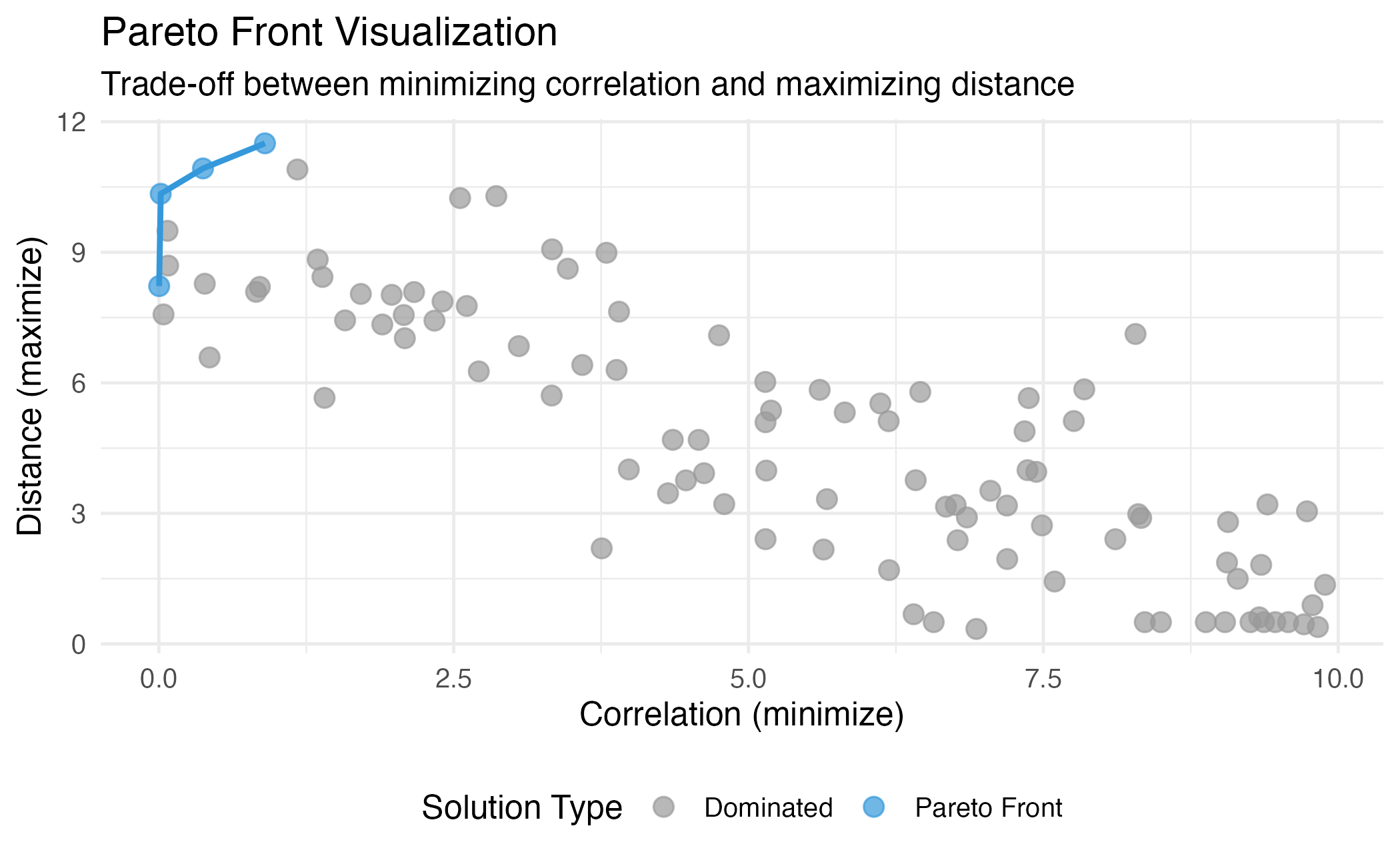

Illustration of Pareto dominance and the Pareto front. Points on the front (blue) are non-dominated.

NSGA-II Algorithm

darwin implements NSGA-II (Non-dominated Sorting Genetic Algorithm II), a widely-used evolutionary algorithm for multi-objective optimization.

Algorithm Overview

Algorithm: NSGA-II
Input: Population size N, generations G, objectives f₁...fₘ
Output: Pareto-optimal gene subsets

1. Initialize population P₀ with N random gene selections
2. Evaluate objectives for all individuals
3. For generation t = 1 to G:
   a. Create offspring Q_t using selection, crossover, mutation
   b. Combine: R_t = P_t ∪ Q_t
   c. Non-dominated sorting of R_t into fronts F₁, F₂, ...
   d. Select N individuals for P_{t+1} using fronts and crowding distance
4. Return final Pareto front

Key Components

1. Non-dominated Sorting

Individuals are sorted into fronts based on dominance:

Front 1: All non-dominated individuals
Front 2: Non-dominated among remaining individuals
Front k: Continue until all individuals are assigned

# Simulate fitness values
set.seed(123)
n <- 20
fitness <- matrix(runif(n * 2), ncol = 2)
colnames(fitness) <- c("Obj1", "Obj2")

# Non-dominated sorting (simplified)
ranks <- darwin:::.non_dominated_sort(-fitness)  # Negate for maximization

df_fronts <- data.frame(
  Obj1 = fitness[, 1],
  Obj2 = fitness[, 2],
  Front = factor(ranks)
)

ggplot(df_fronts, aes(x = Obj1, y = Obj2, color = Front, shape = Front)) +
  geom_point(size = 4) +
  scale_color_brewer(palette = "Set1") +
  labs(
    title = "Non-dominated Sorting",
    subtitle = "Individuals assigned to Pareto fronts",
    x = "Objective 1",
    y = "Objective 2"
  ) +
  theme_minimal(base_size = 12)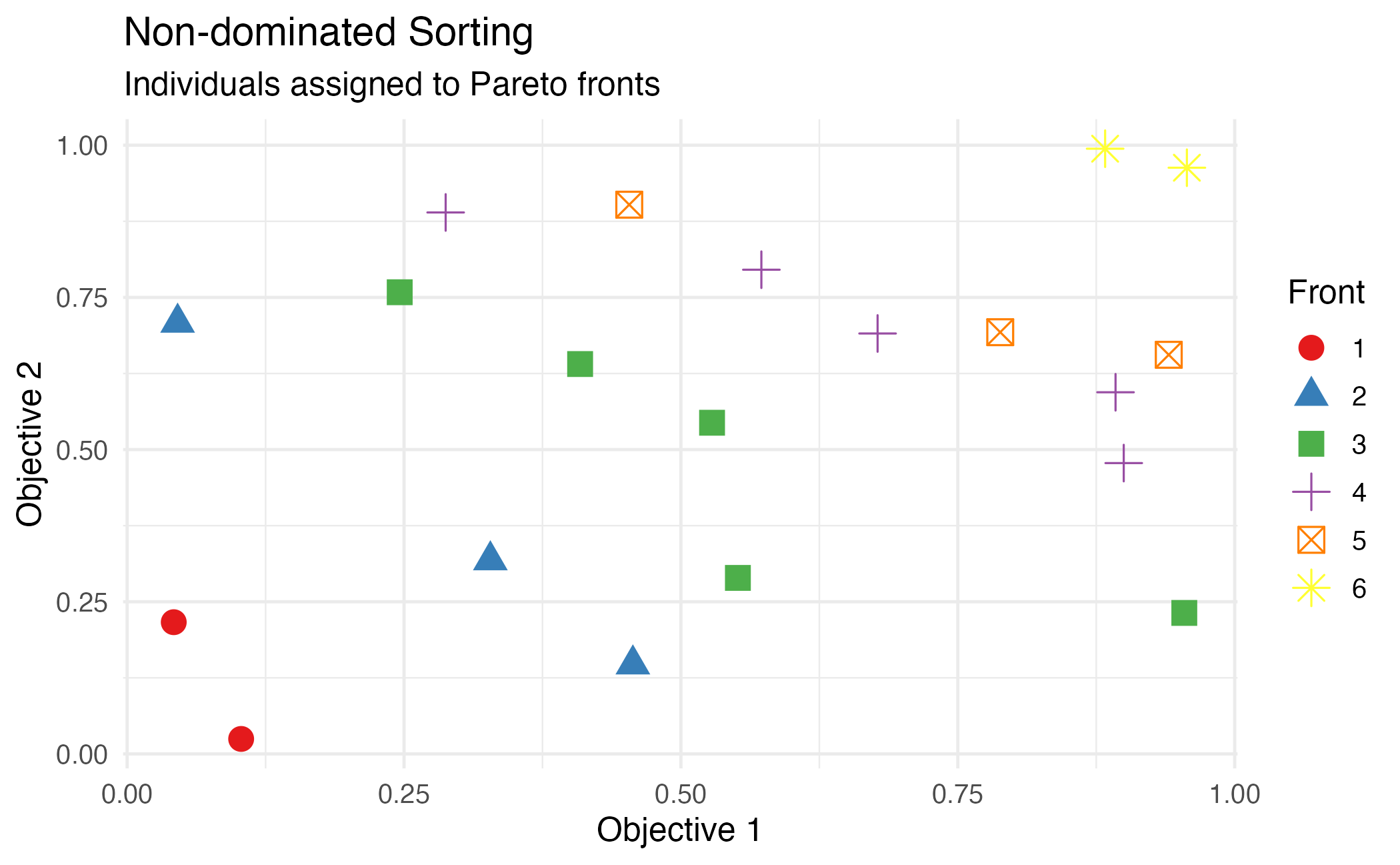

Non-dominated sorting assigns individuals to Pareto fronts.

2. Crowding Distance

Within each front, crowding distance measures the density of solutions around each individual. Higher crowding distance indicates more isolated solutions, which are preferred to maintain diversity.

For individual $i$ in front $F$ :

$d_i = \sum_{m=1}^{M} \frac{f_m^{i+1} - f_m^{i-1}}{f_m^{max} - f_m^{min}}$

where $f_m^{i+1}$ and $f_m^{i-1}$ are the objective values of neighboring individuals when sorted by objective $m$ .

set.seed(456)
n <- 15
f1 <- sort(runif(n, 1, 10))
f2 <- 10 - f1 + rnorm(n, sd = 0.3)

fitness_mat <- cbind(f1, f2)
crowding <- crowding_distance(fitness_mat, ranks = rep(1, n))
crowding[is.infinite(crowding)] <- max(crowding[is.finite(crowding)]) * 1.5

df_crowd <- data.frame(f1 = f1, f2 = f2, crowding = crowding)

ggplot(df_crowd, aes(x = f1, y = f2, size = crowding, color = crowding)) +
  geom_point(alpha = 0.8) +
  scale_size_continuous(range = c(3, 10)) +
  scale_color_gradient(low = "#3498db", high = "#e74c3c") +
  labs(
    title = "Crowding Distance Visualization",
    subtitle = "Larger points = higher crowding distance (more isolated)",
    x = "Objective 1",
    y = "Objective 2",
    size = "Crowding\nDistance",
    color = "Crowding\nDistance"
  ) +
  theme_minimal(base_size = 12)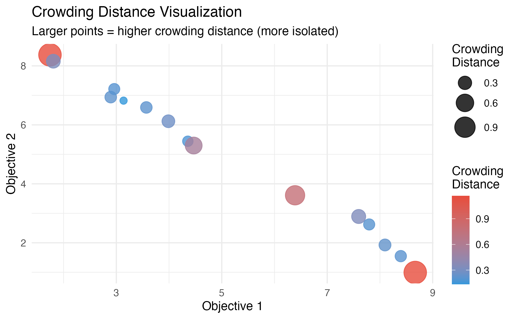

Crowding distance computation. Boundary solutions receive infinite distance.

3. Selection

Selection combines front rank and crowding distance:

Prefer individuals with better (lower) front rank
Within the same front, prefer higher crowding distance

4. Genetic Operators

Crossover: darwin uses two crossover strategies:

AND/OR crossover (early generations): child1 = parent1 AND parent2, child2 = parent1 OR parent2
Two-point crossover (later generations): Standard segment exchange

Mutation: Bit-flip mutation with probability $p_{mut}$ per gene:

$P(\text{flip gene } g) = p_{mut}$

Objective Functions

Correlation Objective (Minimize)

Measures the total pairwise correlation between cell type expression profiles:

$f_{corr}(S) = \sum_{i < j} |\rho_{ij}|$

where $\rho_{ij}$ is the Pearson correlation coefficient between cell types $i$ and $j$ .

Intuition: Low correlation ensures cell types are distinguishable, improving deconvolution accuracy.

library(darwin)
set.seed(42)

# Create data with structure
n_ct <- 5
n_genes <- 100
data <- matrix(rnorm(n_ct * n_genes), nrow = n_ct)
rownames(data) <- paste0("CT", 1:n_ct)

# Add markers
for (i in 1:n_ct) {
  data[i, ((i-1)*10+1):(i*10)] <- data[i, ((i-1)*10+1):(i*10)] + 3
}

# Compute correlation
corr_mat <- cor(t(data))

# Plot
df_corr <- expand.grid(CT1 = rownames(corr_mat), CT2 = colnames(corr_mat))
df_corr$correlation <- as.vector(corr_mat)

ggplot(df_corr, aes(x = CT1, y = CT2, fill = correlation)) +
  geom_tile() +
  scale_fill_gradient2(low = "#3498db", mid = "white", high = "#e74c3c", midpoint = 0) +
  labs(
    title = "Cell Type Correlation Matrix",
    subtitle = paste("Total absolute correlation:", round(compute_correlation(data), 2)),
    x = "", y = ""
  ) +
  theme_minimal(base_size = 12) +
  coord_fixed()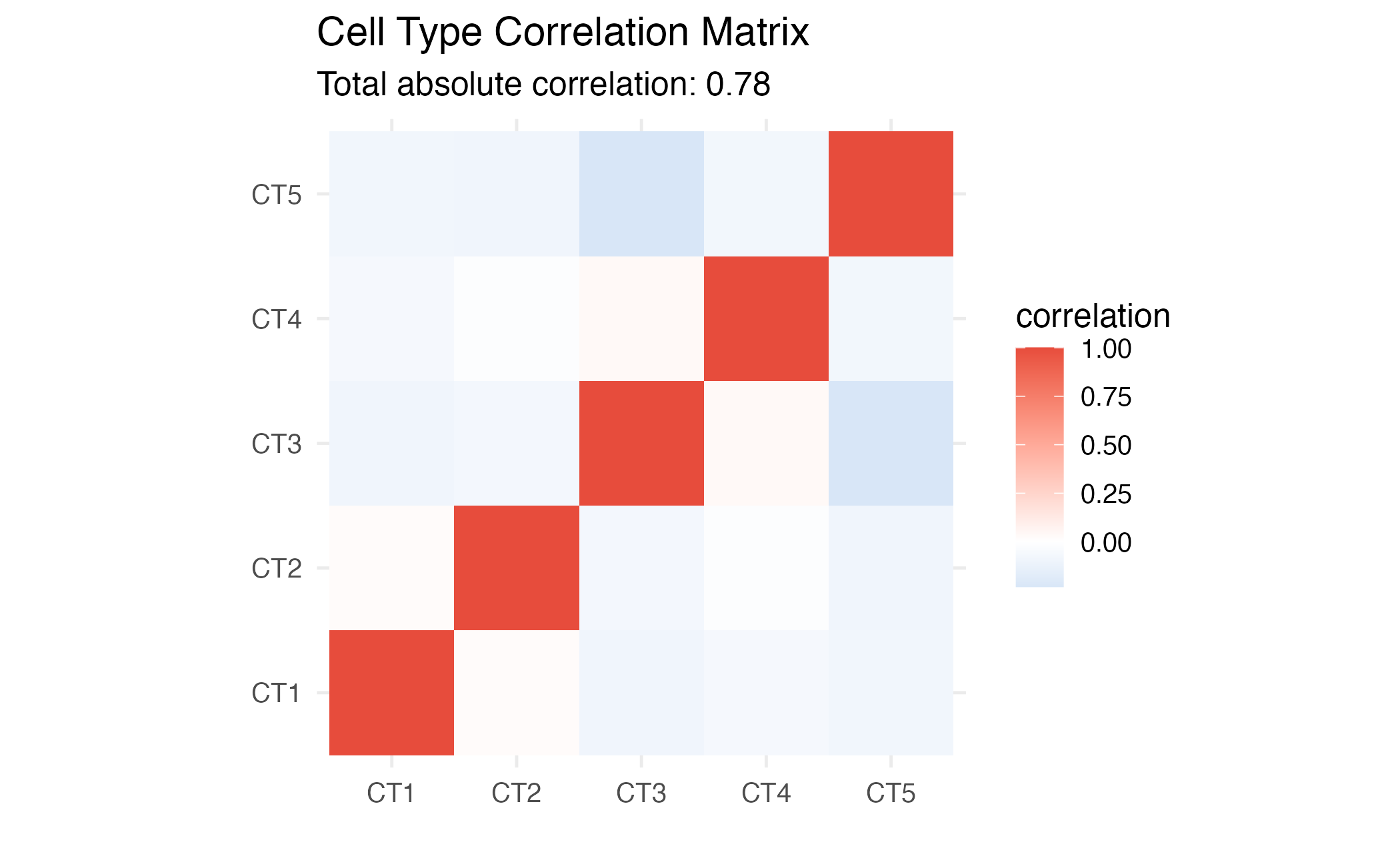

Correlation matrix heatmap for selected genes.

Distance Objective (Maximize)

Measures the total pairwise Euclidean distance between cell type profiles:

$f_{dist}(S) = \sum_{i < j} \|\mathbf{x}_i - \mathbf{x}_j\|_2$

Intuition: Large distances ensure cell type profiles are well-separated in gene expression space.

Condition Number (Minimize)

For deconvolution stability, the condition number of the reference matrix is important:

$\kappa(\mathbf{X}) = \frac{\sigma_{max}}{\sigma_{min}}$

A high condition number indicates potential numerical instability in deconvolution.

Parameter Guidelines

Parameter	Typical Range	Effect
`ngen`	50-500	More generations = better convergence, longer runtime
`pop_size`	50-200	Larger = more diversity, slower
`mutation_prob`	0.001-0.01	Higher = more exploration
`crossover_prob`	0.6-0.9	Higher = more recombination

References

NSGA-II: Deb, K., Pratap, A., Agarwal, S., & Meyarivan, T. (2002). A fast and elitist multiobjective genetic algorithm: NSGA-II. IEEE Transactions on Evolutionary Computation, 6(2), 182-197.
AutoGeneS: Aliee, H., & Theis, F. J. (2021). AutoGeneS: Automatic gene selection using multi-objective optimization for RNA-seq deconvolution. Cell Systems, 12(7), 706-715.e4.

Session Info

sessionInfo()
#> R version 4.4.0 (2024-04-24)
#> Platform: aarch64-apple-darwin20
#> Running under: macOS 15.6.1
#> 
#> Matrix products: default
#> BLAS:   /Library/Frameworks/R.framework/Versions/4.4-arm64/Resources/lib/libRblas.0.dylib 
#> LAPACK: /Library/Frameworks/R.framework/Versions/4.4-arm64/Resources/lib/libRlapack.dylib;  LAPACK version 3.12.0
#> 
#> locale:
#> [1] C
#> 
#> time zone: Asia/Shanghai
#> tzcode source: internal
#> 
#> attached base packages:
#> [1] stats     graphics  grDevices utils     datasets  methods   base     
#> 
#> other attached packages:
#> [1] ggplot2_4.0.1 darwin_1.0.0 
#> 
#> loaded via a namespace (and not attached):
#>  [1] sass_0.4.10         future_1.69.0       generics_0.1.4     
#>  [4] lattice_0.22-7      listenv_0.10.0      digest_0.6.39      
#>  [7] magrittr_2.0.4      evaluate_1.0.5      grid_4.4.0         
#> [10] RColorBrewer_1.1-3  fastmap_1.2.0       jsonlite_2.0.0     
#> [13] Matrix_1.7-4        scales_1.4.0        codetools_0.2-20   
#> [16] textshaping_1.0.4   jquerylib_0.1.4     cli_3.6.5          
#> [19] rlang_1.1.7         parallelly_1.46.1   future.apply_1.20.1
#> [22] withr_3.0.2         cachem_1.1.0        yaml_2.3.12        
#> [25] otel_0.2.0          tools_4.4.0         parallel_4.4.0     
#> [28] dplyr_1.1.4         globals_0.18.0      vctrs_0.7.1        
#> [31] R6_2.6.1            lifecycle_1.0.5     fs_1.6.6           
#> [34] htmlwidgets_1.6.4   ragg_1.5.0          pkgconfig_2.0.3    
#> [37] desc_1.4.3          pkgdown_2.1.3       pillar_1.11.1      
#> [40] bslib_0.9.0         gtable_0.3.6        glue_1.8.0         
#> [43] Rcpp_1.1.1          systemfonts_1.3.1   xfun_0.56          
#> [46] tibble_3.3.1        tidyselect_1.2.1    knitr_1.51         
#> [49] dichromat_2.0-0.1   farver_2.1.2        htmltools_0.5.9    
#> [52] rmarkdown_2.30      labeling_0.4.3      compiler_4.4.0     
#> [55] S7_0.2.1

Zaoqu Liu

2026-01-25