Bulk RNA-seq Deconvolution

Introduction

Bulk RNA-seq deconvolution is the computational process of estimating cell type proportions from bulk tissue transcriptomic data. This vignette demonstrates how to use darwin for the complete deconvolution workflow.

The Deconvolution Problem

Mathematical Formulation

The bulk expression of a tissue sample can be modeled as a weighted sum of cell type expression profiles:

$\mathbf{b} = \mathbf{X} \cdot \mathbf{p} + \boldsymbol{\epsilon}$

where: - $\mathbf{b} \in \mathbb{R}^n$ : Bulk expression vector (n genes) - $\mathbf{X} \in \mathbb{R}^{n \times k}$ : Reference signature matrix (n genes × k cell types) - $\mathbf{p} \in \mathbb{R}^k$ : Cell type proportions to estimate - $\boldsymbol{\epsilon}$ : Noise term

Why Gene Selection Matters

The choice of genes significantly impacts deconvolution accuracy:

Too few genes: Insufficient information for accurate estimation
Too many genes: Noise and uninformative genes degrade performance
Correlated genes: Multicollinearity leads to unstable estimates

darwin addresses this by selecting genes that minimize correlation while maximizing cell type separability.

Complete Workflow

Step 1: Load Package and Data

library(darwin)
library(ggplot2)

set.seed(42)

Step 2: Create Reference Matrix

In practice, this would come from single-cell RNA-seq data.

# Simulate reference data: 8 cell types × 500 genes
n_celltypes <- 8
n_genes <- 500

cell_types <- c("B_cells", "CD4_T", "CD8_T", "NK", "Monocytes", 
                "Dendritic", "Macrophages", "Neutrophils")

reference <- matrix(
  abs(rnorm(n_celltypes * n_genes, mean = 3, sd = 1.5)),
  nrow = n_celltypes,
  ncol = n_genes
)
rownames(reference) <- cell_types
colnames(reference) <- paste0("Gene", 1:n_genes)

# Add cell-type specific marker expression
marker_strength <- c(5, 4, 4, 4.5, 3.5, 4, 3.5, 3)
for (i in 1:n_celltypes) {
  markers <- ((i - 1) * 20 + 1):(i * 20)
  reference[i, markers] <- reference[i, markers] + marker_strength[i]
}

cat("Reference matrix dimensions:", dim(reference), "\n")
#> Reference matrix dimensions: 8 500

Step 3: Create Simulated Bulk Data

We create bulk samples with known cell type proportions for validation.

# True proportions for 10 samples
n_samples <- 10
true_proportions <- matrix(0, nrow = n_samples, ncol = n_celltypes)
colnames(true_proportions) <- cell_types
rownames(true_proportions) <- paste0("Sample", 1:n_samples)

# Generate random proportions that sum to 1
for (i in 1:n_samples) {
  props <- runif(n_celltypes)
  true_proportions[i, ] <- props / sum(props)
}

# Generate bulk expression: bulk = proportions %*% reference + noise
bulk <- true_proportions %*% reference
bulk <- bulk + matrix(rnorm(n_samples * n_genes, sd = 0.5), nrow = n_samples)
bulk[bulk < 0] <- 0

cat("Bulk matrix dimensions:", dim(bulk), "\n")
#> Bulk matrix dimensions: 10 500
cat("\nTrue proportions (first 3 samples):\n")
#> 
#> True proportions (first 3 samples):
print(round(true_proportions[1:3, ], 3))
#>         B_cells CD4_T CD8_T    NK Monocytes Dendritic Macrophages Neutrophils
#> Sample1   0.122 0.090 0.057 0.053     0.102     0.199       0.178       0.199
#> Sample2   0.007 0.022 0.045 0.274     0.175     0.165       0.039       0.274
#> Sample3   0.228 0.039 0.042 0.149     0.053     0.112       0.112       0.265

Step 4: Optimize Gene Selection

# Initialize darwin
dw <- darwin(reference)

# Run multi-objective optimization
dw$optimize(
  ngen = 100,
  pop_size = 80,
  objectives = c("correlation", "distance"),
  weights = c(-1, 1),
  verbose = FALSE,
  parallel = FALSE
)

# Visualize Pareto front
dw$plot()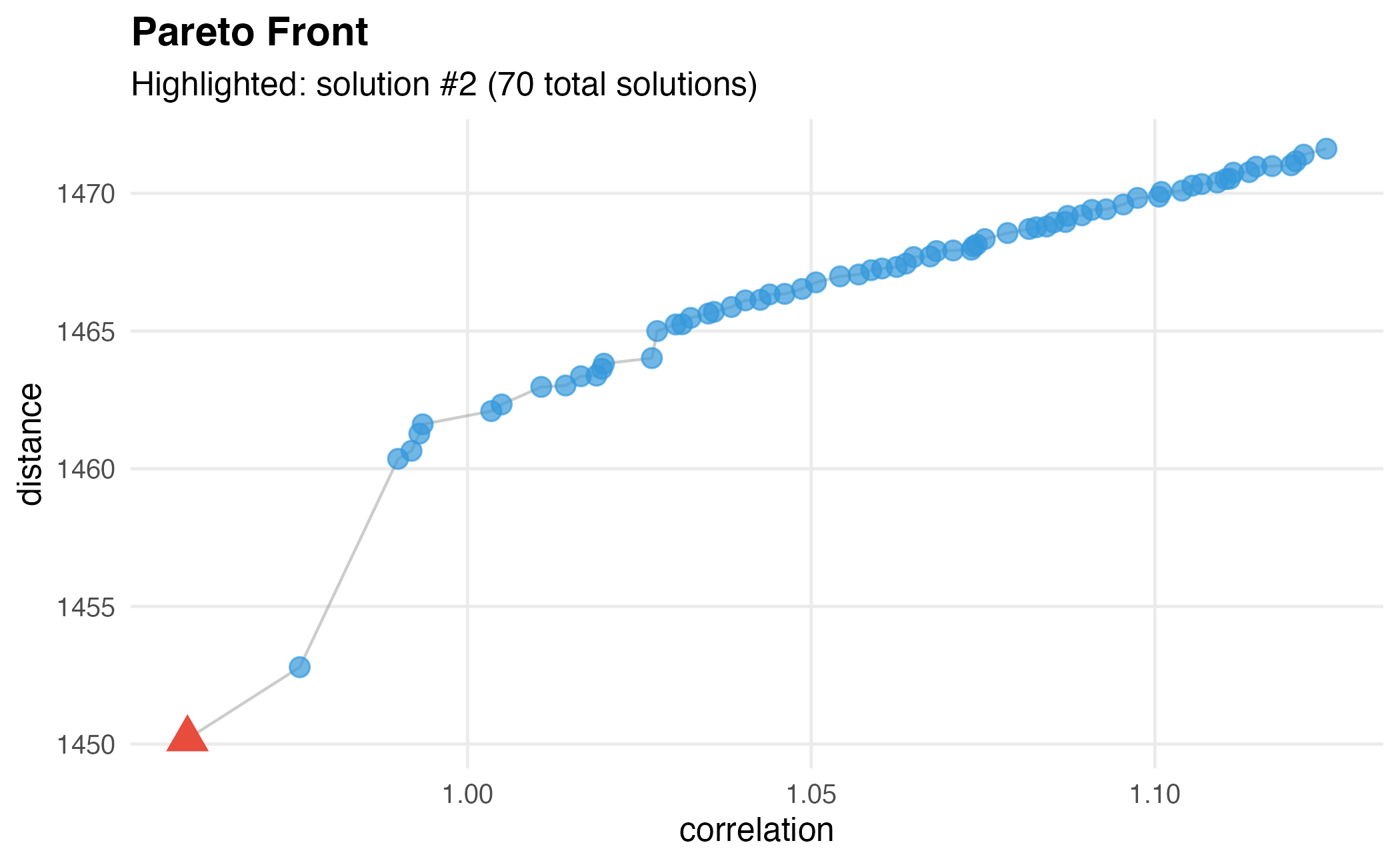

Step 5: Select Optimal Genes

# Select solution balancing both objectives
dw$select(weights = c(-1, 1))

# Check selection statistics
genes <- dw$get_genes()
selection <- dw$get_selection()

cat("Selected", length(genes), "genes\n")
#> Selected 489 genes
cat("Correlation score:", round(compute_correlation(reference[, selection]), 3), "\n")
#> Correlation score: 0.959
cat("Distance score:", round(compute_distance(reference[, selection]), 3), "\n")
#> Distance score: 1450.187

Step 6: Perform Deconvolution

darwin supports three deconvolution methods:

Non-Negative Least Squares (NNLS)

result_nnls <- dw$deconvolve(bulk, method = "nnls")

cat("Estimated proportions (NNLS):\n")
#> Estimated proportions (NNLS):
print(round(result_nnls$proportions[1:3, ], 3))
#>         B_cells CD4_T CD8_T    NK Monocytes Dendritic Macrophages Neutrophils
#> Sample1   0.103 0.091 0.065 0.073     0.118     0.189       0.164       0.196
#> Sample2   0.001 0.037 0.055 0.270     0.189     0.163       0.026       0.258
#> Sample3   0.211 0.038 0.056 0.160     0.056     0.114       0.116       0.249

Linear Regression

result_linear <- dw$deconvolve(bulk, method = "linear")

cat("Estimated proportions (Linear):\n")
#> Estimated proportions (Linear):
print(round(result_linear$proportions[1:3, ], 3))
#>         B_cells CD4_T CD8_T    NK Monocytes Dendritic Macrophages Neutrophils
#> Sample1   0.103 0.091 0.065 0.073     0.118     0.189       0.164       0.196
#> Sample2   0.001 0.037 0.055 0.270     0.189     0.163       0.026       0.258
#> Sample3   0.211 0.038 0.056 0.160     0.056     0.114       0.116       0.249

Step 7: Evaluate Accuracy

# Compare estimated to true proportions
estimated <- result_nnls$proportions

# Calculate correlation per cell type
correlations <- sapply(1:n_celltypes, function(i) {
  cor(true_proportions[, i], estimated[, i])
})
names(correlations) <- cell_types

# Calculate RMSE per cell type
rmse <- sapply(1:n_celltypes, function(i) {
  sqrt(mean((true_proportions[, i] - estimated[, i])^2))
})
names(rmse) <- cell_types

# Summary table
accuracy <- data.frame(
  CellType = cell_types,
  Correlation = round(correlations, 3),
  RMSE = round(rmse, 4)
)
knitr::kable(accuracy, caption = "Deconvolution accuracy by cell type")

Deconvolution accuracy by cell type
	CellType	Correlation	RMSE
B_cells	B_cells	0.984	0.0152
CD4_T	CD4_T	0.994	0.0158
CD8_T	CD8_T	0.996	0.0094
NK	NK	0.986	0.0142
Monocytes	Monocytes	0.994	0.0108
Dendritic	Dendritic	0.971	0.0136
Macrophages	Macrophages	0.987	0.0135
Neutrophils	Neutrophils	0.990	0.0100

# Create comparison data frame
df_compare <- data.frame(
  True = as.vector(true_proportions),
  Estimated = as.vector(estimated),
  CellType = rep(cell_types, each = n_samples),
  Sample = rep(rownames(true_proportions), n_celltypes)
)

# Overall correlation
overall_cor <- cor(df_compare$True, df_compare$Estimated)

ggplot(df_compare, aes(x = True, y = Estimated, color = CellType)) +
  geom_point(size = 2, alpha = 0.7) +
  geom_abline(intercept = 0, slope = 1, linetype = "dashed", color = "gray40") +
  scale_color_brewer(palette = "Set2") +
  labs(
    title = "True vs Estimated Cell Type Proportions",
    subtitle = paste("Overall Pearson r =", round(overall_cor, 3)),
    x = "True Proportion",
    y = "Estimated Proportion",
    color = "Cell Type"
  ) +
  theme_minimal(base_size = 12) +
  coord_fixed(xlim = c(0, 0.4), ylim = c(0, 0.4))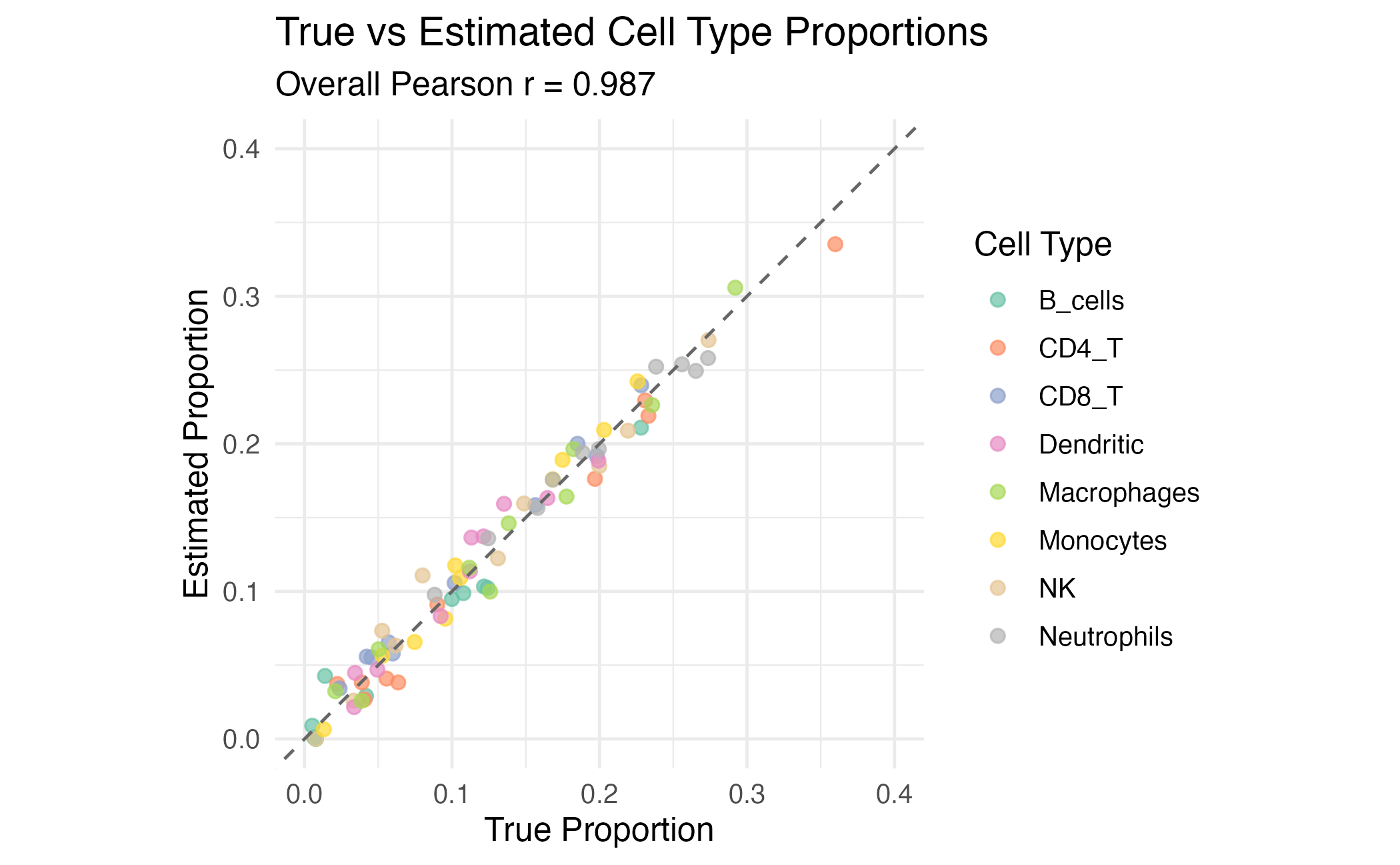

Scatter plot of true vs estimated proportions for each cell type.

ggplot(df_compare, aes(x = True, y = Estimated)) +
  geom_point(color = "#3498db", alpha = 0.7) +
  geom_abline(intercept = 0, slope = 1, linetype = "dashed", color = "#e74c3c") +
  facet_wrap(~CellType, scales = "free") +
  labs(
    title = "Deconvolution Accuracy by Cell Type",
    x = "True Proportion",
    y = "Estimated Proportion"
  ) +
  theme_minimal(base_size = 10)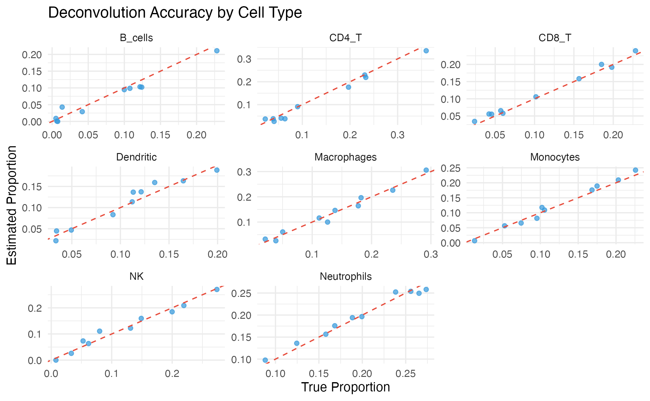

Per-cell-type comparison of true vs estimated proportions.

Comparing Gene Selection Strategies

# Strategy 1: All genes
all_genes_cor <- sapply(1:n_celltypes, function(i) {
  # Deconvolve with all genes (simplified)
  X <- t(reference)
  y <- t(bulk)
  coef_mat <- solve(t(X) %*% X) %*% t(X) %*% y
  estimated_all <- t(coef_mat)
  estimated_all <- estimated_all / rowSums(abs(estimated_all))
  cor(true_proportions[, i], estimated_all[, i])
})

# Strategy 2: darwin selected genes
darwin_cor <- correlations

# Strategy 3: Random genes (same number)
n_selected <- sum(selection)
set.seed(123)
random_selection <- sample(1:n_genes, n_selected)
X_random <- t(reference[, random_selection])
y_random <- t(bulk[, random_selection])
coef_random <- solve(t(X_random) %*% X_random) %*% t(X_random) %*% y_random
estimated_random <- t(coef_random)
estimated_random <- estimated_random / rowSums(abs(estimated_random))
random_cor <- sapply(1:n_celltypes, function(i) {
  cor(true_proportions[, i], estimated_random[, i])
})

# Compare
comparison <- data.frame(
  CellType = rep(cell_types, 3),
  Correlation = c(all_genes_cor, darwin_cor, random_cor),
  Strategy = rep(c("All Genes", "darwin", "Random"), each = n_celltypes)
)

ggplot(comparison, aes(x = CellType, y = Correlation, fill = Strategy)) +
  geom_bar(stat = "identity", position = "dodge") +
  scale_fill_manual(values = c("#95a5a6", "#3498db", "#e74c3c")) +
  labs(
    title = "Deconvolution Accuracy by Gene Selection Strategy",
    x = "Cell Type",
    y = "Correlation (True vs Estimated)"
  ) +
  theme_minimal(base_size = 12) +
  theme(axis.text.x = element_text(angle = 45, hjust = 1)) +
  coord_cartesian(ylim = c(0, 1))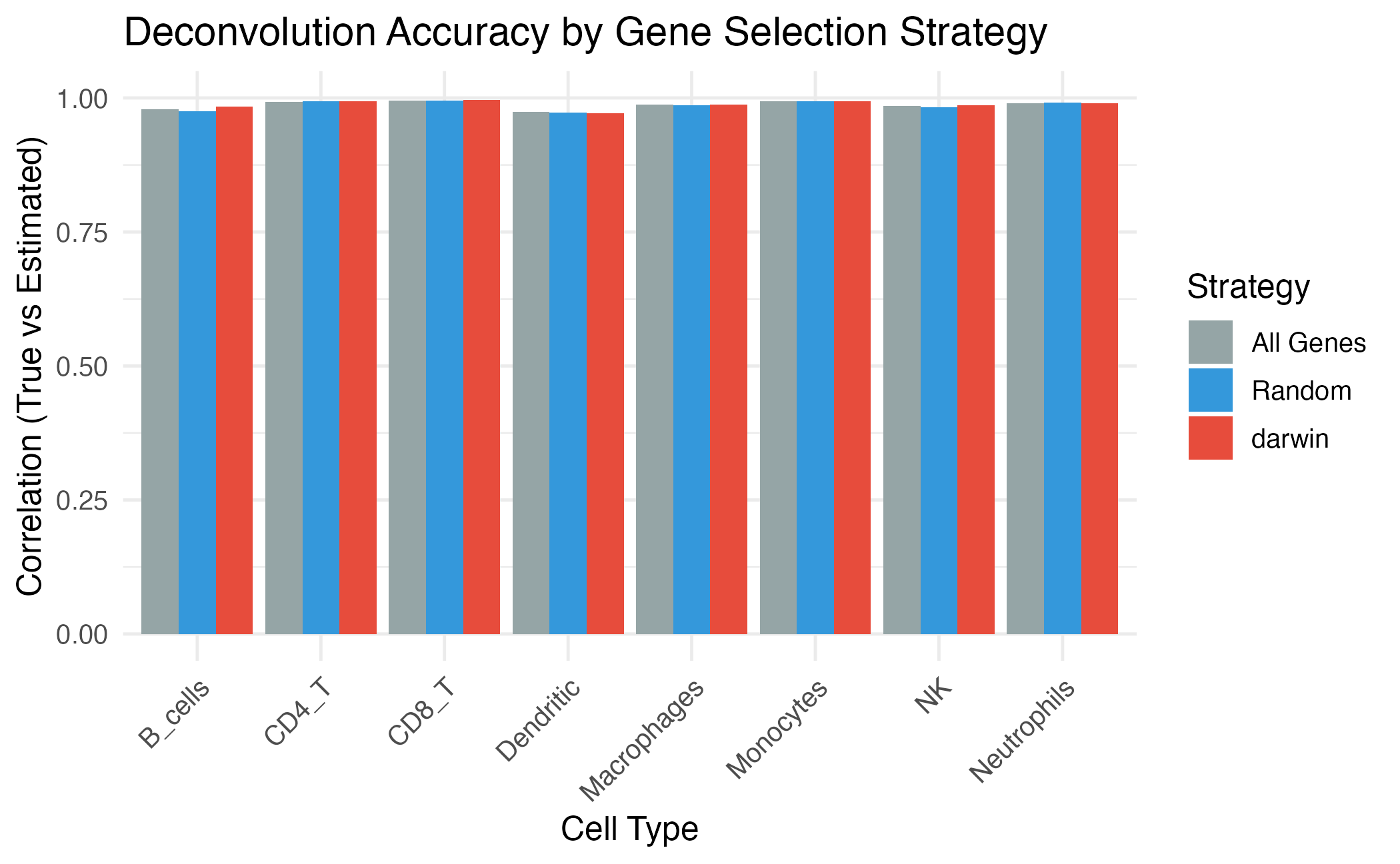

Impact of gene selection on deconvolution accuracy.

Best Practices

1. Reference Matrix Quality

Use high-quality single-cell reference data
Ensure all relevant cell types are represented
Consider batch effects between reference and bulk data

2. Gene Selection

Run optimization with sufficient generations (≥100)
Compare multiple solutions from the Pareto front
Validate with known mixtures when possible

3. Method Selection

Method	Advantages	Disadvantages
NNLS	Non-negative estimates	May underestimate
NuSVR	Robust to outliers	Requires tuning
Linear	Fast, analytical	May give negative values

4. Validation

Use in silico mixtures for benchmarking
Cross-validate with flow cytometry when available
Check that proportions sum to approximately 1

Session Info

sessionInfo()
#> R version 4.4.0 (2024-04-24)
#> Platform: aarch64-apple-darwin20
#> Running under: macOS 15.6.1
#> 
#> Matrix products: default
#> BLAS:   /Library/Frameworks/R.framework/Versions/4.4-arm64/Resources/lib/libRblas.0.dylib 
#> LAPACK: /Library/Frameworks/R.framework/Versions/4.4-arm64/Resources/lib/libRlapack.dylib;  LAPACK version 3.12.0
#> 
#> locale:
#> [1] C
#> 
#> time zone: Asia/Shanghai
#> tzcode source: internal
#> 
#> attached base packages:
#> [1] stats     graphics  grDevices utils     datasets  methods   base     
#> 
#> other attached packages:
#> [1] ggplot2_4.0.1 darwin_1.0.0 
#> 
#> loaded via a namespace (and not attached):
#>  [1] sass_0.4.10         future_1.69.0       generics_0.1.4     
#>  [4] lattice_0.22-7      listenv_0.10.0      digest_0.6.39      
#>  [7] magrittr_2.0.4      evaluate_1.0.5      grid_4.4.0         
#> [10] RColorBrewer_1.1-3  fastmap_1.2.0       jsonlite_2.0.0     
#> [13] Matrix_1.7-4        scales_1.4.0        codetools_0.2-20   
#> [16] textshaping_1.0.4   jquerylib_0.1.4     cli_3.6.5          
#> [19] rlang_1.1.7         parallelly_1.46.1   future.apply_1.20.1
#> [22] withr_3.0.2         cachem_1.1.0        yaml_2.3.12        
#> [25] otel_0.2.0          tools_4.4.0         parallel_4.4.0     
#> [28] dplyr_1.1.4         globals_0.18.0      vctrs_0.7.1        
#> [31] R6_2.6.1            lifecycle_1.0.5     fs_1.6.6           
#> [34] htmlwidgets_1.6.4   ragg_1.5.0          pkgconfig_2.0.3    
#> [37] desc_1.4.3          pkgdown_2.1.3       pillar_1.11.1      
#> [40] bslib_0.9.0         gtable_0.3.6        glue_1.8.0         
#> [43] Rcpp_1.1.1          systemfonts_1.3.1   xfun_0.56          
#> [46] tibble_3.3.1        tidyselect_1.2.1    knitr_1.51         
#> [49] dichromat_2.0-0.1   farver_2.1.2        htmltools_0.5.9    
#> [52] rmarkdown_2.30      labeling_0.4.3      compiler_4.4.0     
#> [55] S7_0.2.1            nnls_1.6

Zaoqu Liu

2026-01-25